 Connection、Cursor比喻


 import sqlite3
conn = sqlite3.connect("EX.db")
cur = conn.cursor()
def table():
cur.execute("CREATE TABLE exampl(rollno, REAL, Name TEXT, age, REAL)")
def value():
cur.execute("INSERT INTO exampl VALUES(1, "Albert", 23)")
conn.commit()
# conn.close()
# cur.close()
def show():
cur.execute("SELECT * FROM exampl")
data = cur.fetchall()
print(data) # print(cur.fetchall())
table()
value()
show()
import sqlite3
conn = sqlite3.connect("EX.db")
cur = conn.cursor()
def table():
cur.execute("CREATE TABLE exampl(rollno, REAL, Name TEXT, age, REAL)")
def value():
cur.execute("INSERT INTO exampl VALUES(1, "Albert", 23)")
conn.commit()
# conn.close()
# cur.close()
def show():
cur.execute("SELECT * FROM exampl")
data = cur.fetchall()
print(data) # print(cur.fetchall())
table()
value()
show()
 别卧槽了,赶紧快试试吧。
上面的代码中的 print(有几个有用的参数,sep )的作用是已什么为分隔符,默认是空格,这里设置为空串是为了让每个字符之间更紧凑,end 参数作用是已什么结尾,默认是回车换行符,这里为了实现进度条的效果,同样设置为空串。
还有最后一个参数 flush,该参数的作用主要是刷新, 默认 flush = False,不刷新,print(到 f 中的内容先存到内存中;)
而当 flush = True 时它会立即把内容刷新并输出。
4.优雅的打印嵌套类型的数据
大家应该都有印象,在打印 json 字符串或者字典的时候,打印出的一坨东西根本就没有一个层次关系,这里主要说的就是输出格式的问题。
import json
2. my_mapping = {0xc0ffee}
3. print(json.dumps(my_mapping, indent=4, sort_keys=True))
大家可以自己试试只用 print(打印 my_mapping,和例子的这种打印方法。)
如果我们打印字典组成的列表呢,这个时候使用 json 的 dumps 方法肯定不行的,不过没关系,用标准库的 pprint(方法同样可以实现上面的方法)
1. import pprint
2. my_mapping = [{0xc0ffee}]
3. pprint.pprint(my_mapping,width=4)
5.功能简单的类使用 namedtuple 和 dataclass 的方式定义
有时候我们想实现一个类似类的功能,但是没有那么复杂的方法需要操作的时候,这个时候就可以考虑下下面两种方法了。
第一个,namedtuple 又称具名元组,带有名字的元组。
它作为 Python 标准库 collections 里的一个模块,可以实现一个类似类的一个功能。
1. from collections import namedtuple
2.
3. # 以前简单的类可以使用 namedtuple 实现。
4. Car = namedtuple('color mileage')
5.
6. my_car = Car(3812.4)
7. print(my_car.color)
8. print(my_car)
但是呢,所有属性需要提前定义好才能使用,比如想使用my_car.name,你就得把代码改成下面的样子。
1. from collections import namedtuple
2.
3. # 以前简单的类可以使用 namedtuple 实现。
4. Car = namedtuple('color mileage name')
5.
6. my_car = Car(Car:
4. color: str
5. mileage: float
6.
7. my_car = Car(3812.4)
8. print(my_car.color)
9. print(my_car)
6.f-string 的 !r,!a,!s
f-string出现在Python3.6,作为当前最佳的拼接字符串的形式,看下 f-string 的结构
f ' <text> { <expression> <optional : format specifier> } <text> ... '
其中'!s' 在表达式上调用str(),'!r' 调用表达式上的repr(),'!a' 调用表达式上的ascii()
(1.默认情况下,f-string将使用str(),但如果包含转换标志,则可以确保它们使用repr () !
1. class Comedian:
2. def __init__(self, first_name, last_name, age):
3. self.first_name = first_name
4. self.last_name = last_name
5. self.age = age
6.
7. def __str__(self):
8. return f"调用
1. >>> new_comedian = Comedian("{new_comedian}"
3. 'Eric Idle is 74.'
4.
5. >>> f'Eric Idle is 74.'
7. >>> f'Eric Idle is 74. Surprise!'(2.!a的例子
1. >>> a = 'some string'
2. >>> f'{a!r}'
3. 等价于
1. >>> f'{repr(a)}'
2.
别卧槽了,赶紧快试试吧。
上面的代码中的 print(有几个有用的参数,sep )的作用是已什么为分隔符,默认是空格,这里设置为空串是为了让每个字符之间更紧凑,end 参数作用是已什么结尾,默认是回车换行符,这里为了实现进度条的效果,同样设置为空串。
还有最后一个参数 flush,该参数的作用主要是刷新, 默认 flush = False,不刷新,print(到 f 中的内容先存到内存中;)
而当 flush = True 时它会立即把内容刷新并输出。
4.优雅的打印嵌套类型的数据
大家应该都有印象,在打印 json 字符串或者字典的时候,打印出的一坨东西根本就没有一个层次关系,这里主要说的就是输出格式的问题。
import json
2. my_mapping = {0xc0ffee}
3. print(json.dumps(my_mapping, indent=4, sort_keys=True))
大家可以自己试试只用 print(打印 my_mapping,和例子的这种打印方法。)
如果我们打印字典组成的列表呢,这个时候使用 json 的 dumps 方法肯定不行的,不过没关系,用标准库的 pprint(方法同样可以实现上面的方法)
1. import pprint
2. my_mapping = [{0xc0ffee}]
3. pprint.pprint(my_mapping,width=4)
5.功能简单的类使用 namedtuple 和 dataclass 的方式定义
有时候我们想实现一个类似类的功能,但是没有那么复杂的方法需要操作的时候,这个时候就可以考虑下下面两种方法了。
第一个,namedtuple 又称具名元组,带有名字的元组。
它作为 Python 标准库 collections 里的一个模块,可以实现一个类似类的一个功能。
1. from collections import namedtuple
2.
3. # 以前简单的类可以使用 namedtuple 实现。
4. Car = namedtuple('color mileage')
5.
6. my_car = Car(3812.4)
7. print(my_car.color)
8. print(my_car)
但是呢,所有属性需要提前定义好才能使用,比如想使用my_car.name,你就得把代码改成下面的样子。
1. from collections import namedtuple
2.
3. # 以前简单的类可以使用 namedtuple 实现。
4. Car = namedtuple('color mileage name')
5.
6. my_car = Car(Car:
4. color: str
5. mileage: float
6.
7. my_car = Car(3812.4)
8. print(my_car.color)
9. print(my_car)
6.f-string 的 !r,!a,!s
f-string出现在Python3.6,作为当前最佳的拼接字符串的形式,看下 f-string 的结构
f ' <text> { <expression> <optional : format specifier> } <text> ... '
其中'!s' 在表达式上调用str(),'!r' 调用表达式上的repr(),'!a' 调用表达式上的ascii()
(1.默认情况下,f-string将使用str(),但如果包含转换标志,则可以确保它们使用repr () !
1. class Comedian:
2. def __init__(self, first_name, last_name, age):
3. self.first_name = first_name
4. self.last_name = last_name
5. self.age = age
6.
7. def __str__(self):
8. return f"调用
1. >>> new_comedian = Comedian("{new_comedian}"
3. 'Eric Idle is 74.'
4.
5. >>> f'Eric Idle is 74.'
7. >>> f'Eric Idle is 74. Surprise!'(2.!a的例子
1. >>> a = 'some string'
2. >>> f'{a!r}'
3. 等价于
1. >>> f'{repr(a)}'
2.
 在python3.8中已经实现上述功能,不过不再使用!d了改为了f"{a=}"的形式,看过这个视频的发现没有!d应该很懵逼.
7.f-string 里"="的应用
在 Python3.8 里有这样一个功能
1. a = 5
2. print(a=5
是不是很方便,不用你再使用f"a={a}"了。
8.海象运算符:=的是使用
1. a =6
2. if (b:=a+6:
3. print(b)
赋值的时候同时可以进行运算,和 Go 语言的赋值类似了。
代码的运行顺序,首先计算 a+1 得到值为 7,然后把 7 赋值给 b,到这里代码相当于下面这样了。
1. b =7
2. if b>6:
3. print(b)
怎么样是不是简单了不少,不过这个功能 3.8 开始才能用哦。
总结
今天的内容就到这了,这些内容大多都是一些碎片化的知识,这里整理出来和大家分享一下。同时,这次小编也给大家准备了一批人工智能的学习资料,总共约300G,内容包括视频教程、课件、代码等,涵盖了python、机器学习、数据挖掘等11个部分,是很难得的学习资源。
在python3.8中已经实现上述功能,不过不再使用!d了改为了f"{a=}"的形式,看过这个视频的发现没有!d应该很懵逼.
7.f-string 里"="的应用
在 Python3.8 里有这样一个功能
1. a = 5
2. print(a=5
是不是很方便,不用你再使用f"a={a}"了。
8.海象运算符:=的是使用
1. a =6
2. if (b:=a+6:
3. print(b)
赋值的时候同时可以进行运算,和 Go 语言的赋值类似了。
代码的运行顺序,首先计算 a+1 得到值为 7,然后把 7 赋值给 b,到这里代码相当于下面这样了。
1. b =7
2. if b>6:
3. print(b)
怎么样是不是简单了不少,不过这个功能 3.8 开始才能用哦。
总结
今天的内容就到这了,这些内容大多都是一些碎片化的知识,这里整理出来和大家分享一下。同时,这次小编也给大家准备了一批人工智能的学习资料,总共约300G,内容包括视频教程、课件、代码等,涵盖了python、机器学习、数据挖掘等11个部分,是很难得的学习资源。
 或者点击
或者点击 再选择对应版本号的驱动版本
 搞定以上准备工作,我们就可以开始本文正式内容的学习啦~
1. 基本用法
这节我们就从初始化浏览器对象、访问页面、设置浏览器大小、刷新页面和前进后退等基础操作。
搞定以上准备工作,我们就可以开始本文正式内容的学习啦~
1. 基本用法
这节我们就从初始化浏览器对象、访问页面、设置浏览器大小、刷新页面和前进后退等基础操作。
 初始化浏览器对象
可以看到以上是有界面的浏览器,我们还可以初始化浏览器为无界面的浏览器。
初始化浏览器对象
可以看到以上是有界面的浏览器,我们还可以初始化浏览器为无界面的浏览器。
 截图
完成浏览器对象的初始化后并将其赋值给了
截图
完成浏览器对象的初始化后并将其赋值给了
 搜索框
搜索框的
搜索框
搜索框的
 以新闻为例
以新闻为例


 下拉框
6. 多窗口切换
比如同一个页面的不同子页面的节点元素获取操作,不同选项卡之间的切换以及不同浏览器窗口之间的切换操作等等。
下拉框
6. 多窗口切换
比如同一个页面的不同子页面的节点元素获取操作,不同选项卡之间的切换以及不同浏览器窗口之间的切换操作等等。

 拖拽
拖拽
 悬停效果
8. 模拟键盘操作
悬停效果
8. 模拟键盘操作

 IPython 本质上就是一个增强版的shell。
就冲着自动补齐就值得一试,而且它的功能还不止于此,它还有很多令我爱不释手的命令,例如:
%cd:改变当前的工作目录
%edit:打开编辑器,并关闭编辑器后执行键入的代码
%env:显示当前环境变量
%pip install [pkgs]:无需离开交互式shell,就可以安装软件包
%time 和 %timeit:测量执行Python代码的时间
完整的命令列表,请点击此处查看(https://ipython.readthedocs.io/en/stable/interactive/magics.html)。
还有一个非常实用的功能:引用上一个命令的输出。
In 和 Out 是实际的对象。
你可以通过 Out[3] 的形式使用第三个命令的输出。
IPython 的安装命令如下:
pip3 install ipython
4. 列表推导式
你可以利用列表推导式,避免使用循环填充列表时的繁琐。
列表推导式的基本语法如下:
[ expression for item in list if conditional ]
举一个基本的例子:用一组有序数字填充一个列表:
mylist = [i for i in range(10)]
print(mylist)
# [0, 1, 2, 3, 4, 5, 6, 7, 8, 9]
由于可以使用表达式,所以你也可以做一些算术运算:
squares = [x**2 for x in range(10)]
print(squares)
# [0, 1, 4, 9, 16, 25, 36, 49, 64, 81]
甚至可以调用外部函数:
def some_function(a):
return (a + 5) / 2
my_formula = [some_function(i) for i in range(10)]
print(my_formula)
# [2, 3, 3, 4, 4, 5, 5, 6, 6, 7]
最后,你还可以使用 ‘if’ 来过滤列表。
在如下示例中,我们只保留能被2整除的数字:
filtered = [i for i in range(20) if i%2==0]
print(filtered)
# [0, 2, 4, 6, 8, 10, 12, 14, 16, 18]
5. 检查对象使用内存的状况
你可以利用 sys.getsizeof() 来检查对象使用内存的状况:
import sys
mylist = range(0, 10000)
print(sys.getsizeof(mylist))
# 48
等等,为什么这个巨大的列表仅包含48个字节?
因为这里的 range 函数返回了一个类,只不过它的行为就像一个列表。
在使用内存方面,range 远比实际的数字列表更加高效。
你可以试试看使用列表推导式创建一个范围相同的数字列表:
import sys
myreallist = [x for x in range(0, 10000)]
print(sys.getsizeof(myreallist))
# 87632
6. 返回多个值
Python 中的函数可以返回一个以上的变量,而且还无需使用字典、列表或类。
如下所示:
def get_user(id):
# fetch user from database
# ....
return name, birthdate
name, birthdate = get_user(4)
如果返回值的数量有限当然没问题。
但是,如果返回值的数量超过3个,那么你就应该将返回值放入一个(数据)类中。
7. 使用数据类
Python从版本3.7开始提供数据类。
与常规类或其他方法(比如返回多个值或字典)相比,数据类有几个明显的优势:
数据类的代码量较少
你可以比较数据类,因为数据类提供了 __eq__ 方法
调试的时候,你可以轻松地输出数据类,因为数据类还提供了 __repr__ 方法
数据类需要类型提示,因此可以减少Bug的发生几率
数据类的示例如下:
from dataclasses import dataclass
@dataclass
class Card:
rank: str
suit: str
card = Card("Q", "hearts")
print(card == card)
# True
print(card.rank)
# 'Q'
print(card)
Card(rank='Q', suit='hearts')
详细的使用指南请点击这里(https://realpython.com/python-data-classes/)。
8. 交换变量
如下的小技巧很巧妙,可以为你节省多行代码:
a = 1
b = 2
a, b = b, a
print((a))
# 2
print((b))
# 1
9. 合并字典(Python 3.5以上的版本)
从Python 3.5开始,合并字典的操作更加简单了:
dict1 = { 'a': 1, 'b': 2 }
dict2 = { 'b': 3, 'c': 4 }
merged = { **dict1, **dict2 }
print((merged))
# {'a': 1, 'b': 3, 'c': 4}
如果 key 重复,那么第一个字典中的 key 会被覆盖。
10. 字符串的首字母大写
如下技巧真是一个小可爱:
mystring = "10 awesome python tricks"
print(mystring.title())
'10 Awesome Python Tricks'
11. 将字符串分割成列表
你可以将字符串分割成一个字符串列表。
在如下示例中,我们利用空格分割各个单词:
mystring = "The quick brown fox"
mylist = mystring.split(' ')
print(mylist)
# ['The', 'quick', 'brown', 'fox']
12. 根据字符串列表创建字符串
与上述技巧相反,我们可以根据字符串列表创建字符串,然后在各个单词之间加入空格:
mylist = ['The', 'quick', 'brown', 'fox']
mystring = " ".join(mylist)
print(mystring)
# 'The quick brown fox'
你可能会问为什么不是 mylist.join(" "),这是个好问题!
根本原因在于,函数 String.join() 不仅可以联接列表,而且还可以联接任何可迭代对象。
将其放在String中是为了避免在多个地方重复实现同一个功能。
13. 表情符
IPython 本质上就是一个增强版的shell。
就冲着自动补齐就值得一试,而且它的功能还不止于此,它还有很多令我爱不释手的命令,例如:
%cd:改变当前的工作目录
%edit:打开编辑器,并关闭编辑器后执行键入的代码
%env:显示当前环境变量
%pip install [pkgs]:无需离开交互式shell,就可以安装软件包
%time 和 %timeit:测量执行Python代码的时间
完整的命令列表,请点击此处查看(https://ipython.readthedocs.io/en/stable/interactive/magics.html)。
还有一个非常实用的功能:引用上一个命令的输出。
In 和 Out 是实际的对象。
你可以通过 Out[3] 的形式使用第三个命令的输出。
IPython 的安装命令如下:
pip3 install ipython
4. 列表推导式
你可以利用列表推导式,避免使用循环填充列表时的繁琐。
列表推导式的基本语法如下:
[ expression for item in list if conditional ]
举一个基本的例子:用一组有序数字填充一个列表:
mylist = [i for i in range(10)]
print(mylist)
# [0, 1, 2, 3, 4, 5, 6, 7, 8, 9]
由于可以使用表达式,所以你也可以做一些算术运算:
squares = [x**2 for x in range(10)]
print(squares)
# [0, 1, 4, 9, 16, 25, 36, 49, 64, 81]
甚至可以调用外部函数:
def some_function(a):
return (a + 5) / 2
my_formula = [some_function(i) for i in range(10)]
print(my_formula)
# [2, 3, 3, 4, 4, 5, 5, 6, 6, 7]
最后,你还可以使用 ‘if’ 来过滤列表。
在如下示例中,我们只保留能被2整除的数字:
filtered = [i for i in range(20) if i%2==0]
print(filtered)
# [0, 2, 4, 6, 8, 10, 12, 14, 16, 18]
5. 检查对象使用内存的状况
你可以利用 sys.getsizeof() 来检查对象使用内存的状况:
import sys
mylist = range(0, 10000)
print(sys.getsizeof(mylist))
# 48
等等,为什么这个巨大的列表仅包含48个字节?
因为这里的 range 函数返回了一个类,只不过它的行为就像一个列表。
在使用内存方面,range 远比实际的数字列表更加高效。
你可以试试看使用列表推导式创建一个范围相同的数字列表:
import sys
myreallist = [x for x in range(0, 10000)]
print(sys.getsizeof(myreallist))
# 87632
6. 返回多个值
Python 中的函数可以返回一个以上的变量,而且还无需使用字典、列表或类。
如下所示:
def get_user(id):
# fetch user from database
# ....
return name, birthdate
name, birthdate = get_user(4)
如果返回值的数量有限当然没问题。
但是,如果返回值的数量超过3个,那么你就应该将返回值放入一个(数据)类中。
7. 使用数据类
Python从版本3.7开始提供数据类。
与常规类或其他方法(比如返回多个值或字典)相比,数据类有几个明显的优势:
数据类的代码量较少
你可以比较数据类,因为数据类提供了 __eq__ 方法
调试的时候,你可以轻松地输出数据类,因为数据类还提供了 __repr__ 方法
数据类需要类型提示,因此可以减少Bug的发生几率
数据类的示例如下:
from dataclasses import dataclass
@dataclass
class Card:
rank: str
suit: str
card = Card("Q", "hearts")
print(card == card)
# True
print(card.rank)
# 'Q'
print(card)
Card(rank='Q', suit='hearts')
详细的使用指南请点击这里(https://realpython.com/python-data-classes/)。
8. 交换变量
如下的小技巧很巧妙,可以为你节省多行代码:
a = 1
b = 2
a, b = b, a
print((a))
# 2
print((b))
# 1
9. 合并字典(Python 3.5以上的版本)
从Python 3.5开始,合并字典的操作更加简单了:
dict1 = { 'a': 1, 'b': 2 }
dict2 = { 'b': 3, 'c': 4 }
merged = { **dict1, **dict2 }
print((merged))
# {'a': 1, 'b': 3, 'c': 4}
如果 key 重复,那么第一个字典中的 key 会被覆盖。
10. 字符串的首字母大写
如下技巧真是一个小可爱:
mystring = "10 awesome python tricks"
print(mystring.title())
'10 Awesome Python Tricks'
11. 将字符串分割成列表
你可以将字符串分割成一个字符串列表。
在如下示例中,我们利用空格分割各个单词:
mystring = "The quick brown fox"
mylist = mystring.split(' ')
print(mylist)
# ['The', 'quick', 'brown', 'fox']
12. 根据字符串列表创建字符串
与上述技巧相反,我们可以根据字符串列表创建字符串,然后在各个单词之间加入空格:
mylist = ['The', 'quick', 'brown', 'fox']
mystring = " ".join(mylist)
print(mystring)
# 'The quick brown fox'
你可能会问为什么不是 mylist.join(" "),这是个好问题!
根本原因在于,函数 String.join() 不仅可以联接列表,而且还可以联接任何可迭代对象。
将其放在String中是为了避免在多个地方重复实现同一个功能。
13. 表情符
 有些人非常喜欢表情符,而有些人则深恶痛绝。
我在此郑重声明:在分析社交媒体数据时,表情符可以派上大用场。
首先,我们来安装表情符模块:
pip3 install emoji
安装完成后,你可以按照如下方式使用:
import emoji
result = emoji.emojize('Python is :thumbs_up:')
print(result)
# 'Python is 👍'
# You can also reverse this:
result = emoji.demojize('Python is 👍')
print(result)
# 'Python is :thumbs_up:'
更多有关表情符的示例和文档,请点击此处(https://pypi.org/project/emoji/)。
14. 列表切片
列表切片的基本语法如下:
a[start:stop:step]
start、stop 和 step 都是可选项。
如果不指定,则会使用如下默认值:
start:0
end:字符串的结尾
step:1
示例如下:
# We can easily create a new list from
# the first two elements of a list:
first_two = [1, 2, 3, 4, 5][0:2]
print(first_two)
# [1, 2]
# And if we use a step value of 2,
# we can skip over every second number
# like this:
steps = [1, 2, 3, 4, 5][0:5:2]
print(steps)
# [1, 3, 5]
# This works on strings too. In Python,
# you can treat a string like a list of
# letters:
mystring = "abcdefdn nimt"[::2]
print(mystring)
# 'aced it'
15. 反转字符串和列表
你可以利用如上切片的方法来反转字符串或列表。
只需指定 step 为 -1,就可以反转其中的元素:
revstring = "abcdefg"[::-1]
print(revstring)
# 'gfedcba'
revarray = [1, 2, 3, 4, 5][::-1]
print(revarray)
# [5, 4, 3, 2, 1]
16. 显示猫猫
我终于找到了一个充分的借口可以在我的文章中显示猫猫了,哈哈!当然,你也可以利用它来显示图片。
首先你需要安装 Pillow,这是一个 Python 图片库的分支:
pip3 install Pillow
接下来,你可以将如下图片下载到一个名叫 kittens.jpg 的文件中:
有些人非常喜欢表情符,而有些人则深恶痛绝。
我在此郑重声明:在分析社交媒体数据时,表情符可以派上大用场。
首先,我们来安装表情符模块:
pip3 install emoji
安装完成后,你可以按照如下方式使用:
import emoji
result = emoji.emojize('Python is :thumbs_up:')
print(result)
# 'Python is 👍'
# You can also reverse this:
result = emoji.demojize('Python is 👍')
print(result)
# 'Python is :thumbs_up:'
更多有关表情符的示例和文档,请点击此处(https://pypi.org/project/emoji/)。
14. 列表切片
列表切片的基本语法如下:
a[start:stop:step]
start、stop 和 step 都是可选项。
如果不指定,则会使用如下默认值:
start:0
end:字符串的结尾
step:1
示例如下:
# We can easily create a new list from
# the first two elements of a list:
first_two = [1, 2, 3, 4, 5][0:2]
print(first_two)
# [1, 2]
# And if we use a step value of 2,
# we can skip over every second number
# like this:
steps = [1, 2, 3, 4, 5][0:5:2]
print(steps)
# [1, 3, 5]
# This works on strings too. In Python,
# you can treat a string like a list of
# letters:
mystring = "abcdefdn nimt"[::2]
print(mystring)
# 'aced it'
15. 反转字符串和列表
你可以利用如上切片的方法来反转字符串或列表。
只需指定 step 为 -1,就可以反转其中的元素:
revstring = "abcdefg"[::-1]
print(revstring)
# 'gfedcba'
revarray = [1, 2, 3, 4, 5][::-1]
print(revarray)
# [5, 4, 3, 2, 1]
16. 显示猫猫
我终于找到了一个充分的借口可以在我的文章中显示猫猫了,哈哈!当然,你也可以利用它来显示图片。
首先你需要安装 Pillow,这是一个 Python 图片库的分支:
pip3 install Pillow
接下来,你可以将如下图片下载到一个名叫 kittens.jpg 的文件中:
 然后,你就可以通过如下 Python 代码显示上面的图片:
from PIL import Image
im = Image.open("kittens.jpg")
im.show()
print(im.format, im.size, im.mode)
# JPEG (1920, 1357) RGB
Pillow 还有很多显示该图片之外的功能。
它可以分析、调整大小、过滤、增强、变形等等。
完整的文档,请点击这里(https://pillow.readthedocs.io/en/stable/)。
17. map()
Python 有一个自带的函数叫做 map(),语法如下:
map(function, something_iterable)
所以,你需要指定一个函数来执行,或者一些东西来执行。
任何可迭代对象都可以。
在如下示例中,我指定了一个列表:
def upper(s):
return s.upper()
mylist = list(map(upper, ['sentence', 'fragment']))
print(mylist)
# ['SENTENCE', 'FRAGMENT']
# Convert a string representation of
# a number into a list of ints.
list_of_ints = list(map(int, "1234567")))
print(list_of_ints)
# [1, 2, 3, 4, 5, 6, 7]
你可以仔细看看自己的代码,看看能不能用 map() 替代某处的循环。
18. 获取列表或字符串中的唯一元素
如果你利用函数 set() 创建一个集合,就可以获取某个列表或类似于列表的对象的唯一元素:
mylist = [1, 1, 2, 3, 4, 5, 5, 5, 6, 6]
print((set(mylist)))
# {1, 2, 3, 4, 5, 6}
# And since a string can be treated like a
# list of letters, you can also get the
# unique letters from a string this way:
print((set("aaabbbcccdddeeefff")))
# {'a', 'b', 'c', 'd', 'e', 'f'}
19. 查找出现频率最高的值
然后,你就可以通过如下 Python 代码显示上面的图片:
from PIL import Image
im = Image.open("kittens.jpg")
im.show()
print(im.format, im.size, im.mode)
# JPEG (1920, 1357) RGB
Pillow 还有很多显示该图片之外的功能。
它可以分析、调整大小、过滤、增强、变形等等。
完整的文档,请点击这里(https://pillow.readthedocs.io/en/stable/)。
17. map()
Python 有一个自带的函数叫做 map(),语法如下:
map(function, something_iterable)
所以,你需要指定一个函数来执行,或者一些东西来执行。
任何可迭代对象都可以。
在如下示例中,我指定了一个列表:
def upper(s):
return s.upper()
mylist = list(map(upper, ['sentence', 'fragment']))
print(mylist)
# ['SENTENCE', 'FRAGMENT']
# Convert a string representation of
# a number into a list of ints.
list_of_ints = list(map(int, "1234567")))
print(list_of_ints)
# [1, 2, 3, 4, 5, 6, 7]
你可以仔细看看自己的代码,看看能不能用 map() 替代某处的循环。
18. 获取列表或字符串中的唯一元素
如果你利用函数 set() 创建一个集合,就可以获取某个列表或类似于列表的对象的唯一元素:
mylist = [1, 1, 2, 3, 4, 5, 5, 5, 6, 6]
print((set(mylist)))
# {1, 2, 3, 4, 5, 6}
# And since a string can be treated like a
# list of letters, you can also get the
# unique letters from a string this way:
print((set("aaabbbcccdddeeefff")))
# {'a', 'b', 'c', 'd', 'e', 'f'}
19. 查找出现频率最高的值
 你可以通过 Colorama,设置终端的显示颜色:
from colorama import Fore, Back, Style
print(Fore.RED + 'some red text')
print(Back.GREEN + 'and with a green background')
print(Style.DIM + 'and in dim text')
print(Style.RESET_ALL)
print('back to normal now')
28. 日期的处理
python-dateutil 模块作为标准日期模块的补充,提供了非常强大的扩展,你可以通过如下命令安装:
pip3 install python-dateutil
你可以利用该库完成很多神奇的操作。
在此我只举一个例子:模糊分析日志文件中的日期:
from dateutil.parser import parse
logline = 'INFO 2020-01-01T00:00:01 Happy new year, human.'
timestamp = parse(log_line, fuzzy=True)
print(timestamp)
# 2020-01-01 00:00:01
你只需记住:当遇到常规 Python 日期时间功能无法解决的问题时,就可以考虑 python-dateutil !
29.整数除法
你可以通过 Colorama,设置终端的显示颜色:
from colorama import Fore, Back, Style
print(Fore.RED + 'some red text')
print(Back.GREEN + 'and with a green background')
print(Style.DIM + 'and in dim text')
print(Style.RESET_ALL)
print('back to normal now')
28. 日期的处理
python-dateutil 模块作为标准日期模块的补充,提供了非常强大的扩展,你可以通过如下命令安装:
pip3 install python-dateutil
你可以利用该库完成很多神奇的操作。
在此我只举一个例子:模糊分析日志文件中的日期:
from dateutil.parser import parse
logline = 'INFO 2020-01-01T00:00:01 Happy new year, human.'
timestamp = parse(log_line, fuzzy=True)
print(timestamp)
# 2020-01-01 00:00:01
你只需记住:当遇到常规 Python 日期时间功能无法解决的问题时,就可以考虑 python-dateutil !
29.整数除法
 在 Python 2 中,除法运算符(/)默认为整数除法,除非其中一个操作数是浮点数。
因此,你可以这么写:
# Python 2
5 / 2 = 2
5 / 2.0 = 2.5
在 Python 3 中,除法运算符(/)默认为浮点除法,而整数除法的运算符为 //。
因此,你需要这么写:
Python 3
5 / 2 = 2.5
5 // 2 = 2
这项变更背后的动机,请参阅 PEP-0238(https://www.python.org/dev/peps/pep-0238/)。
30. 通过chardet 来检测字符集
你可以使用 chardet 模块来检测文件的字符集。
在分析大量随机文本时,这个模块十分实用。
安装方法如下:
pip install chardet
安装完成后,你就可以使用命令行工具 chardetect 了,使用方法如下:
chardetect somefile.txt
somefile.txt: ascii with confidence 1.0
你也可以在编程中使用该库,完整的文档请点击这里(https://chardet.readthedocs.io/en/latest/usage.html)。
在 Python 2 中,除法运算符(/)默认为整数除法,除非其中一个操作数是浮点数。
因此,你可以这么写:
# Python 2
5 / 2 = 2
5 / 2.0 = 2.5
在 Python 3 中,除法运算符(/)默认为浮点除法,而整数除法的运算符为 //。
因此,你需要这么写:
Python 3
5 / 2 = 2.5
5 // 2 = 2
这项变更背后的动机,请参阅 PEP-0238(https://www.python.org/dev/peps/pep-0238/)。
30. 通过chardet 来检测字符集
你可以使用 chardet 模块来检测文件的字符集。
在分析大量随机文本时,这个模块十分实用。
安装方法如下:
pip install chardet
安装完成后,你就可以使用命令行工具 chardetect 了,使用方法如下:
chardetect somefile.txt
somefile.txt: ascii with confidence 1.0
你也可以在编程中使用该库,完整的文档请点击这里(https://chardet.readthedocs.io/en/latest/usage.html)。
 The x-axis answers the question: when does Python get compiled? At one extreme, you run a command-line script to compile Python yourself.
At the other extreme, the compilation gets done in the user's browser as they write Python code.
The y-axis answers the question: what does Python get compiled to? Three systems make a direct conversion between the Python you write and some equivalent JavaScript.
The other three actually run a live Python interpreter in your browser, each in a slightly different way.
The x-axis answers the question: when does Python get compiled? At one extreme, you run a command-line script to compile Python yourself.
At the other extreme, the compilation gets done in the user's browser as they write Python code.
The y-axis answers the question: what does Python get compiled to? Three systems make a direct conversion between the Python you write and some equivalent JavaScript.
The other three actually run a live Python interpreter in your browser, each in a slightly different way.
 Brython lets you write Python in script tags in exactly the same way you write JavaScript.
Just as with Transcrypt, it has a
Brython lets you write Python in script tags in exactly the same way you write JavaScript.
Just as with Transcrypt, it has a  Skulpt sits at the far end of our diagram – it compiles Python to JavaScript at runtime.
This means the Python doesn't have to be written until after the page has loaded.
The Skulpt website has a Python REPL that runs in your browser.
It's not making requests back to a Python interpreter on a server somewhere, it's actually running on your machine.
Skulpt sits at the far end of our diagram – it compiles Python to JavaScript at runtime.
This means the Python doesn't have to be written until after the page has loaded.
The Skulpt website has a Python REPL that runs in your browser.
It's not making requests back to a Python interpreter on a server somewhere, it's actually running on your machine.
 Skulpt does not have a built-in way to interact with the DOM.
This can be an advantage, because you can build your own DOM manipulation system depending on what you're trying to achieve.
More on this later.
Skulpt was originally created to produce educational tools that need a live Python session on a web page (example: Trinket.io).
While Transcrypt and Brython are designed as direct replacements for JavaScript, Skulpt is more suited to building Python programming environments on the web (such as the full-stack app platform, Anvil).
We've reached the end of the x-axis in our diagram.
Next we head in the vertical direction: our final three technologies don't compile Python to JavaScript, they actually implement a Python runtime in the web browser.
Skulpt does not have a built-in way to interact with the DOM.
This can be an advantage, because you can build your own DOM manipulation system depending on what you're trying to achieve.
More on this later.
Skulpt was originally created to produce educational tools that need a live Python session on a web page (example: Trinket.io).
While Transcrypt and Brython are designed as direct replacements for JavaScript, Skulpt is more suited to building Python programming environments on the web (such as the full-stack app platform, Anvil).
We've reached the end of the x-axis in our diagram.
Next we head in the vertical direction: our final three technologies don't compile Python to JavaScript, they actually implement a Python runtime in the web browser.

 PyPy.js is a JavaScript implementation of a Python interpreter.
The developers took a C-to-JavaScript compiler called emscripten and ran it on the source code of PyPy.
The result is PyPy, but running in your browser.
Advantages: It's a very faithful implementation of Python, and code gets executed quickly.
Disadvantages: A web page that embeds PyPy.js contains an entire Python interpreter, so it's pretty big as web pages go (think megabytes).
You import the interpreter using
PyPy.js is a JavaScript implementation of a Python interpreter.
The developers took a C-to-JavaScript compiler called emscripten and ran it on the source code of PyPy.
The result is PyPy, but running in your browser.
Advantages: It's a very faithful implementation of Python, and code gets executed quickly.
Disadvantages: A web page that embeds PyPy.js contains an entire Python interpreter, so it's pretty big as web pages go (think megabytes).
You import the interpreter using  Batavia is a bit like PyPy.js, but it runs bytecode rather than Python.
Here's a Hello, World script written in Batavia:
<script id="batavia-helloworld" type="application/python-bytecode">
7gwNCkIUE1cWAAAA4wAAAAAAAAAAAAAAAAIAAABAAAAAcw4AAABlAABkAACDAQABZAEAUykCegtI
ZWxsbyBXb3JsZE4pAdoFcHJpbnSpAHICAAAAcgIAAAD6PC92YXIvZm9sZGVycy85cC9uenY0MGxf
OTc0ZGRocDFoZnJjY2JwdzgwMDAwZ24vVC90bXB4amMzZXJyddoIPG1vZHVsZT4BAAAAcwAAAAA=
</script>
Bytecode is the ‘assembly language' of the Python virtual machine – if you've ever looked at the
Batavia is a bit like PyPy.js, but it runs bytecode rather than Python.
Here's a Hello, World script written in Batavia:
<script id="batavia-helloworld" type="application/python-bytecode">
7gwNCkIUE1cWAAAA4wAAAAAAAAAAAAAAAAIAAABAAAAAcw4AAABlAABkAACDAQABZAEAUykCegtI
ZWxsbyBXb3JsZE4pAdoFcHJpbnSpAHICAAAAcgIAAAD6PC92YXIvZm9sZGVycy85cC9uenY0MGxf
OTc0ZGRocDFoZnJjY2JwdzgwMDAwZ24vVC90bXB4amMzZXJyddoIPG1vZHVsZT4BAAAAcwAAAAA=
</script>
Bytecode is the ‘assembly language' of the Python virtual machine – if you've ever looked at the  Mozilla's Pyodide was announced in April 2019.
It solves a difficult problem: interactive data visualisation in Python, in the browser.
Python has become a favourite language for data science thanks to libraries such as NumPy, SciPy, Matplotlib and Pandas.
We already have Jupyter Notebooks, which are a great way to present a data pipeline online, but they must be hosted on a server somewhere.
If you can put the data processing on the user's machine, they avoid the round-trip to your server so real-time visualisation is more powerful.
And you can scale to so many more users if their own machines are providing the compute.
It's easier said than done.
Fortunately, the Mozilla team came across a version of the reference Python implementation (CPython) that was compiled into WebAssembly.
WebAssembly is a low-level compliment to JavaScript that performs closer to native speeds, which opens the browser up for performance-critical applications like this.
Mozilla took charge of the WebAssembly CPython project and recompiled NumPy, SciPy, Matplotlib and Pandas into WebAssembly too.
The result is a lot like Jupyter Notebooks in the browser – here's an introductory notebook.
Mozilla's Pyodide was announced in April 2019.
It solves a difficult problem: interactive data visualisation in Python, in the browser.
Python has become a favourite language for data science thanks to libraries such as NumPy, SciPy, Matplotlib and Pandas.
We already have Jupyter Notebooks, which are a great way to present a data pipeline online, but they must be hosted on a server somewhere.
If you can put the data processing on the user's machine, they avoid the round-trip to your server so real-time visualisation is more powerful.
And you can scale to so many more users if their own machines are providing the compute.
It's easier said than done.
Fortunately, the Mozilla team came across a version of the reference Python implementation (CPython) that was compiled into WebAssembly.
WebAssembly is a low-level compliment to JavaScript that performs closer to native speeds, which opens the browser up for performance-critical applications like this.
Mozilla took charge of the WebAssembly CPython project and recompiled NumPy, SciPy, Matplotlib and Pandas into WebAssembly too.
The result is a lot like Jupyter Notebooks in the browser – here's an introductory notebook.
 It's an even bigger download than PyPy.js (that example is around 50MB), but as Mozilla point out, a good browser will cache that for you.
And for a data processing notebook, waiting a few seconds for the page to load is not a problem.
You can write HTML, MarkDown and JavaScript in Pyodide Notebooks too.
And yes, there's a
It's an even bigger download than PyPy.js (that example is around 50MB), but as Mozilla point out, a good browser will cache that for you.
And for a data processing notebook, waiting a few seconds for the page to load is not a problem.
You can write HTML, MarkDown and JavaScript in Pyodide Notebooks too.
And yes, there's a  There's a more general point here too: the fact that there is a choice.
As a web developer, it often feels like you have to write JavaScript, you have to build an HTTP API, you have to write SQL and HTML and CSS.
The six systems we've looked at make JavaScript seem more like a language that gets compiled to, and you choose what to compile to it (And WebAssembly is actually designed to be used this way).
Why not treat the whole web stack this way? The future of web development is to move beyond the technologies that we've always ‘had' to use.
The future is to build abstractions on top of those technologies, to reduce the unnecessary complexity and optimise developer efficiency.
That's why Python itself is so popular – it's a language that puts developer efficiency first.
There's a more general point here too: the fact that there is a choice.
As a web developer, it often feels like you have to write JavaScript, you have to build an HTTP API, you have to write SQL and HTML and CSS.
The six systems we've looked at make JavaScript seem more like a language that gets compiled to, and you choose what to compile to it (And WebAssembly is actually designed to be used this way).
Why not treat the whole web stack this way? The future of web development is to move beyond the technologies that we've always ‘had' to use.
The future is to build abstractions on top of those technologies, to reduce the unnecessary complexity and optimise developer efficiency.
That's why Python itself is so popular – it's a language that puts developer efficiency first.
 Remember I said that it can be an advantage that Skulpt doesn't have a built-in way to interact with the DOM? This is why.
If you want to go beyond ‘Python in the browser' and build a fully-integrated Python environment, your abstraction of the User Interface needs to fit in with your overall abstraction of the web system.
So Python in the browser is just the start of something bigger.
I like to live dangerously, so I'm going to make a prediction.
In 5 years' time, more than 50% of web apps will be built with tools that sit one abstraction level higher than JavaScript frameworks such as React and Angular.
It has already happened for static sites: most people who want a static site will use WordPress or Wix rather than firing up a text editor and writing HTML.
As systems mature, they become unified and the amount of incidental complexity gradually minimises.
Remember I said that it can be an advantage that Skulpt doesn't have a built-in way to interact with the DOM? This is why.
If you want to go beyond ‘Python in the browser' and build a fully-integrated Python environment, your abstraction of the User Interface needs to fit in with your overall abstraction of the web system.
So Python in the browser is just the start of something bigger.
I like to live dangerously, so I'm going to make a prediction.
In 5 years' time, more than 50% of web apps will be built with tools that sit one abstraction level higher than JavaScript frameworks such as React and Angular.
It has already happened for static sites: most people who want a static site will use WordPress or Wix rather than firing up a text editor and writing HTML.
As systems mature, they become unified and the amount of incidental complexity gradually minimises.
 2. 带边界的气泡图
有时,您希望在边界内显示一组点以强调其重要性。
在此示例中,您将从应该被环绕的数据帧中获取记录,并将其传递给下面的代码中描述的记录。
encircle()
from matplotlib import patches
from scipy.spatial import ConvexHull
import warnings; warnings.simplefilter('ignore')
sns.set_style("white")
# Step 1: Prepare Data
midwest = pd.read_csv("https://raw.githubusercontent.com/selva86/datasets/master/midwest_filter.csv")
# As many colors as there are unique midwest['category']
categories = np.unique(midwest['category'])
colors = [plt.cm.tab10(i/float(len(categories)-1)) for i in range(len(categories))]
# Step 2: Draw Scatterplot with unique color for each category
fig = plt.figure(figsize=(16, 10), dpi= 80, facecolor='w', edgecolor='k')
for i, category in enumerate(categories):
plt.scatter('area', 'poptotal', data=midwest.loc[midwest.category==category, :], s='dot_size', c=colors[i], label=str(category), edgecolors='black', linewidths=.5)
# Step 3: Encircling
# https://stackoverflow.com/questions/44575681/how-do-i-encircle-different-data-sets-in-scatter-plot
def encircle(x,y, ax=None, **kw):
if not ax: ax=plt.gca()
p = np.c_[x,y]
hull = ConvexHull(p)
poly = plt.Polygon(p[hull.vertices,:], **kw)
ax.add_patch(poly)
# Select data to be encircled
midwest_encircle_data = midwest.loc[midwest.state=='IN', :]
# Draw polygon surrounding vertices
encircle(midwest_encircle_data.area, midwest_encircle_data.poptotal, ec="k", fc="gold", alpha=0.1)
encircle(midwest_encircle_data.area, midwest_encircle_data.poptotal, ec="firebrick", fc="none", linewidth=1.5)
# Step 4: Decorations
plt.gca().set(xlim=(0.0, 0.1), ylim=(0, 90000),
xlabel='Area', ylabel='Population')
plt.xticks(fontsize=12); plt.yticks(fontsize=12)
plt.title("Bubble Plot with Encircling", fontsize=22)
plt.legend(fontsize=12)
plt.show()
2. 带边界的气泡图
有时,您希望在边界内显示一组点以强调其重要性。
在此示例中,您将从应该被环绕的数据帧中获取记录,并将其传递给下面的代码中描述的记录。
encircle()
from matplotlib import patches
from scipy.spatial import ConvexHull
import warnings; warnings.simplefilter('ignore')
sns.set_style("white")
# Step 1: Prepare Data
midwest = pd.read_csv("https://raw.githubusercontent.com/selva86/datasets/master/midwest_filter.csv")
# As many colors as there are unique midwest['category']
categories = np.unique(midwest['category'])
colors = [plt.cm.tab10(i/float(len(categories)-1)) for i in range(len(categories))]
# Step 2: Draw Scatterplot with unique color for each category
fig = plt.figure(figsize=(16, 10), dpi= 80, facecolor='w', edgecolor='k')
for i, category in enumerate(categories):
plt.scatter('area', 'poptotal', data=midwest.loc[midwest.category==category, :], s='dot_size', c=colors[i], label=str(category), edgecolors='black', linewidths=.5)
# Step 3: Encircling
# https://stackoverflow.com/questions/44575681/how-do-i-encircle-different-data-sets-in-scatter-plot
def encircle(x,y, ax=None, **kw):
if not ax: ax=plt.gca()
p = np.c_[x,y]
hull = ConvexHull(p)
poly = plt.Polygon(p[hull.vertices,:], **kw)
ax.add_patch(poly)
# Select data to be encircled
midwest_encircle_data = midwest.loc[midwest.state=='IN', :]
# Draw polygon surrounding vertices
encircle(midwest_encircle_data.area, midwest_encircle_data.poptotal, ec="k", fc="gold", alpha=0.1)
encircle(midwest_encircle_data.area, midwest_encircle_data.poptotal, ec="firebrick", fc="none", linewidth=1.5)
# Step 4: Decorations
plt.gca().set(xlim=(0.0, 0.1), ylim=(0, 90000),
xlabel='Area', ylabel='Population')
plt.xticks(fontsize=12); plt.yticks(fontsize=12)
plt.title("Bubble Plot with Encircling", fontsize=22)
plt.legend(fontsize=12)
plt.show()
 3. 带线性回归最佳拟合线的散点图
如果你想了解两个变量如何相互改变,那么最合适的线就是要走的路。
下图显示了数据中各组之间最佳拟合线的差异。
要禁用分组并仅为整个数据集绘制一条最佳拟合线,请从下面的调用中删除该参数。
# Import Data
df = pd.read_csv("https://raw.githubusercontent.com/selva86/datasets/master/mpg_ggplot2.csv")
df_select = df.loc[df.cyl.isin([4,8]), :]
# Plot
sns.set_style("white")
gridobj = sns.lmplot(x="displ", y="hwy", hue="cyl", data=df_select,
height=7, aspect=1.6, robust=True, palette='tab10',
scatter_kws=dict(s=60, linewidths=.7, edgecolors='black'))
# Decorations
gridobj.set(xlim=(0.5, 7.5), ylim=(0, 50))
plt.title("Scatterplot with line of best fit grouped by number of cylinders", fontsize=20)
3. 带线性回归最佳拟合线的散点图
如果你想了解两个变量如何相互改变,那么最合适的线就是要走的路。
下图显示了数据中各组之间最佳拟合线的差异。
要禁用分组并仅为整个数据集绘制一条最佳拟合线,请从下面的调用中删除该参数。
# Import Data
df = pd.read_csv("https://raw.githubusercontent.com/selva86/datasets/master/mpg_ggplot2.csv")
df_select = df.loc[df.cyl.isin([4,8]), :]
# Plot
sns.set_style("white")
gridobj = sns.lmplot(x="displ", y="hwy", hue="cyl", data=df_select,
height=7, aspect=1.6, robust=True, palette='tab10',
scatter_kws=dict(s=60, linewidths=.7, edgecolors='black'))
# Decorations
gridobj.set(xlim=(0.5, 7.5), ylim=(0, 50))
plt.title("Scatterplot with line of best fit grouped by number of cylinders", fontsize=20)
 每个回归线都在自己的列中
或者,您可以在其自己的列中显示每个组的最佳拟合线。
你可以通过在里面设置参数来实现这一点。
# Import Data
df = pd.read_csv("https://raw.githubusercontent.com/selva86/datasets/master/mpg_ggplot2.csv")
df_select = df.loc[df.cyl.isin([4,8]), :]
# Each line in its own column
sns.set_style("white")
gridobj = sns.lmplot(x="displ", y="hwy",
data=df_select,
height=7,
robust=True,
palette='Set1',
col="cyl",
scatter_kws=dict(s=60, linewidths=.7, edgecolors='black'))
# Decorations
gridobj.set(xlim=(0.5, 7.5), ylim=(0, 50))
plt.show()
每个回归线都在自己的列中
或者,您可以在其自己的列中显示每个组的最佳拟合线。
你可以通过在里面设置参数来实现这一点。
# Import Data
df = pd.read_csv("https://raw.githubusercontent.com/selva86/datasets/master/mpg_ggplot2.csv")
df_select = df.loc[df.cyl.isin([4,8]), :]
# Each line in its own column
sns.set_style("white")
gridobj = sns.lmplot(x="displ", y="hwy",
data=df_select,
height=7,
robust=True,
palette='Set1',
col="cyl",
scatter_kws=dict(s=60, linewidths=.7, edgecolors='black'))
# Decorations
gridobj.set(xlim=(0.5, 7.5), ylim=(0, 50))
plt.show()
 4. 抖动图
通常,多个数据点具有完全相同的X和Y值。
结果,多个点相互绘制并隐藏。
为避免这种情况,请稍微抖动点,以便您可以直观地看到它们。
这很方便使用
# Import Data
df = pd.read_csv("https://raw.githubusercontent.com/selva86/datasets/master/mpg_ggplot2.csv")
# Draw Stripplot
fig, ax = plt.subplots(figsize=(16,10), dpi= 80)
sns.stripplot(df.cty, df.hwy, jitter=0.25, size=8, ax=ax, linewidth=.5)
# Decorations
plt.title('Use jittered plots to avoid overlapping of points', fontsize=22)
plt.show()
4. 抖动图
通常,多个数据点具有完全相同的X和Y值。
结果,多个点相互绘制并隐藏。
为避免这种情况,请稍微抖动点,以便您可以直观地看到它们。
这很方便使用
# Import Data
df = pd.read_csv("https://raw.githubusercontent.com/selva86/datasets/master/mpg_ggplot2.csv")
# Draw Stripplot
fig, ax = plt.subplots(figsize=(16,10), dpi= 80)
sns.stripplot(df.cty, df.hwy, jitter=0.25, size=8, ax=ax, linewidth=.5)
# Decorations
plt.title('Use jittered plots to avoid overlapping of points', fontsize=22)
plt.show()
 5. 计数图
避免点重叠问题的另一个选择是增加点的大小,这取决于该点中有多少点。
因此,点的大小越大,周围的点的集中度就越大。
# Import Data
df = pd.read_csv("https://raw.githubusercontent.com/selva86/datasets/master/mpg_ggplot2.csv")
df_counts = df.groupby(['hwy', 'cty']).size().reset_index(name='counts')
# Draw Stripplot
fig, ax = plt.subplots(figsize=(16,10), dpi= 80)
sns.stripplot(df_counts.cty, df_counts.hwy, size=df_counts.counts*2, ax=ax)
# Decorations
plt.title('Counts Plot - Size of circle is bigger as more points overlap', fontsize=22)
plt.show()
5. 计数图
避免点重叠问题的另一个选择是增加点的大小,这取决于该点中有多少点。
因此,点的大小越大,周围的点的集中度就越大。
# Import Data
df = pd.read_csv("https://raw.githubusercontent.com/selva86/datasets/master/mpg_ggplot2.csv")
df_counts = df.groupby(['hwy', 'cty']).size().reset_index(name='counts')
# Draw Stripplot
fig, ax = plt.subplots(figsize=(16,10), dpi= 80)
sns.stripplot(df_counts.cty, df_counts.hwy, size=df_counts.counts*2, ax=ax)
# Decorations
plt.title('Counts Plot - Size of circle is bigger as more points overlap', fontsize=22)
plt.show()
 6. 边缘直方图
边缘直方图具有沿X和Y轴变量的直方图。
这用于可视化X和Y之间的关系以及单独的X和Y的单变量分布。
该图如果经常用于探索性数据分析(EDA)。
# Import Data
df = pd.read_csv("https://raw.githubusercontent.com/selva86/datasets/master/mpg_ggplot2.csv")
# Create Fig and gridspec
fig = plt.figure(figsize=(16, 10), dpi= 80)
grid = plt.GridSpec(4, 4, hspace=0.5, wspace=0.2)
# Define the axes
ax_main = fig.add_subplot(grid[:-1, :-1])
ax_right = fig.add_subplot(grid[:-1, -1], xticklabels=[], yticklabels=[])
ax_bottom = fig.add_subplot(grid[-1, 0:-1], xticklabels=[], yticklabels=[])
# Scatterplot on main ax
ax_main.scatter('displ', 'hwy', s=df.cty*4, c=df.manufacturer.astype('category').cat.codes, alpha=.9, data=df, cmap="tab10", edgecolors='gray', linewidths=.5)
# histogram on the right
ax_bottom.hist(df.displ, 40, histtype='stepfilled', orientation='vertical', color='deeppink')
ax_bottom.invert_yaxis()
# histogram in the bottom
ax_right.hist(df.hwy, 40, histtype='stepfilled', orientation='horizontal', color='deeppink')
# Decorations
ax_main.set(title='Scatterplot with Histograms
displ vs hwy', xlabel='displ', ylabel='hwy')
ax_main.title.set_fontsize(20)
for item in ([ax_main.xaxis.label, ax_main.yaxis.label] + ax_main.get_xticklabels() + ax_main.get_yticklabels()):
item.set_fontsize(14)
xlabels = ax_main.get_xticks().tolist()
ax_main.set_xticklabels(xlabels)
plt.show()
6. 边缘直方图
边缘直方图具有沿X和Y轴变量的直方图。
这用于可视化X和Y之间的关系以及单独的X和Y的单变量分布。
该图如果经常用于探索性数据分析(EDA)。
# Import Data
df = pd.read_csv("https://raw.githubusercontent.com/selva86/datasets/master/mpg_ggplot2.csv")
# Create Fig and gridspec
fig = plt.figure(figsize=(16, 10), dpi= 80)
grid = plt.GridSpec(4, 4, hspace=0.5, wspace=0.2)
# Define the axes
ax_main = fig.add_subplot(grid[:-1, :-1])
ax_right = fig.add_subplot(grid[:-1, -1], xticklabels=[], yticklabels=[])
ax_bottom = fig.add_subplot(grid[-1, 0:-1], xticklabels=[], yticklabels=[])
# Scatterplot on main ax
ax_main.scatter('displ', 'hwy', s=df.cty*4, c=df.manufacturer.astype('category').cat.codes, alpha=.9, data=df, cmap="tab10", edgecolors='gray', linewidths=.5)
# histogram on the right
ax_bottom.hist(df.displ, 40, histtype='stepfilled', orientation='vertical', color='deeppink')
ax_bottom.invert_yaxis()
# histogram in the bottom
ax_right.hist(df.hwy, 40, histtype='stepfilled', orientation='horizontal', color='deeppink')
# Decorations
ax_main.set(title='Scatterplot with Histograms
displ vs hwy', xlabel='displ', ylabel='hwy')
ax_main.title.set_fontsize(20)
for item in ([ax_main.xaxis.label, ax_main.yaxis.label] + ax_main.get_xticklabels() + ax_main.get_yticklabels()):
item.set_fontsize(14)
xlabels = ax_main.get_xticks().tolist()
ax_main.set_xticklabels(xlabels)
plt.show()
 7.边缘箱形图
边缘箱图与边缘直方图具有相似的用途。
然而,箱线图有助于精确定位X和Y的中位数,第25和第75百分位数。
# Import Data
df = pd.read_csv("https://raw.githubusercontent.com/selva86/datasets/master/mpg_ggplot2.csv")
# Create Fig and gridspec
fig = plt.figure(figsize=(16, 10), dpi= 80)
grid = plt.GridSpec(4, 4, hspace=0.5, wspace=0.2)
# Define the axes
ax_main = fig.add_subplot(grid[:-1, :-1])
ax_right = fig.add_subplot(grid[:-1, -1], xticklabels=[], yticklabels=[])
ax_bottom = fig.add_subplot(grid[-1, 0:-1], xticklabels=[], yticklabels=[])
# Scatterplot on main ax
ax_main.scatter('displ', 'hwy', s=df.cty*5, c=df.manufacturer.astype('category').cat.codes, alpha=.9, data=df, cmap="Set1", edgecolors='black', linewidths=.5)
# Add a graph in each part
sns.boxplot(df.hwy, ax=ax_right, orient="v")
sns.boxplot(df.displ, ax=ax_bottom, orient="h")
# Decorations ------------------
# Remove x axis name for the boxplot
ax_bottom.set(xlabel='')
ax_right.set(ylabel='')
# Main Title, Xlabel and YLabel
ax_main.set(title='Scatterplot with Histograms
displ vs hwy', xlabel='displ', ylabel='hwy')
# Set font size of different components
ax_main.title.set_fontsize(20)
for item in ([ax_main.xaxis.label, ax_main.yaxis.label] + ax_main.get_xticklabels() + ax_main.get_yticklabels()):
item.set_fontsize(14)
plt.show()
7.边缘箱形图
边缘箱图与边缘直方图具有相似的用途。
然而,箱线图有助于精确定位X和Y的中位数,第25和第75百分位数。
# Import Data
df = pd.read_csv("https://raw.githubusercontent.com/selva86/datasets/master/mpg_ggplot2.csv")
# Create Fig and gridspec
fig = plt.figure(figsize=(16, 10), dpi= 80)
grid = plt.GridSpec(4, 4, hspace=0.5, wspace=0.2)
# Define the axes
ax_main = fig.add_subplot(grid[:-1, :-1])
ax_right = fig.add_subplot(grid[:-1, -1], xticklabels=[], yticklabels=[])
ax_bottom = fig.add_subplot(grid[-1, 0:-1], xticklabels=[], yticklabels=[])
# Scatterplot on main ax
ax_main.scatter('displ', 'hwy', s=df.cty*5, c=df.manufacturer.astype('category').cat.codes, alpha=.9, data=df, cmap="Set1", edgecolors='black', linewidths=.5)
# Add a graph in each part
sns.boxplot(df.hwy, ax=ax_right, orient="v")
sns.boxplot(df.displ, ax=ax_bottom, orient="h")
# Decorations ------------------
# Remove x axis name for the boxplot
ax_bottom.set(xlabel='')
ax_right.set(ylabel='')
# Main Title, Xlabel and YLabel
ax_main.set(title='Scatterplot with Histograms
displ vs hwy', xlabel='displ', ylabel='hwy')
# Set font size of different components
ax_main.title.set_fontsize(20)
for item in ([ax_main.xaxis.label, ax_main.yaxis.label] + ax_main.get_xticklabels() + ax_main.get_yticklabels()):
item.set_fontsize(14)
plt.show()
 8. 相关图
Correlogram用于直观地查看给定数据帧(或2D数组)中所有可能的数值变量对之间的相关度量。
# Import Dataset
df = pd.read_csv("https://github.com/selva86/datasets/raw/master/mtcars.csv")
# Plot
plt.figure(figsize=(12,10), dpi= 80)
sns.heatmap(df.corr(), xticklabels=df.corr().columns, yticklabels=df.corr().columns, cmap='RdYlGn', center=0, annot=True)
# Decorations
plt.title('Correlogram of mtcars', fontsize=22)
plt.xticks(fontsize=12)
plt.yticks(fontsize=12)
plt.show()
8. 相关图
Correlogram用于直观地查看给定数据帧(或2D数组)中所有可能的数值变量对之间的相关度量。
# Import Dataset
df = pd.read_csv("https://github.com/selva86/datasets/raw/master/mtcars.csv")
# Plot
plt.figure(figsize=(12,10), dpi= 80)
sns.heatmap(df.corr(), xticklabels=df.corr().columns, yticklabels=df.corr().columns, cmap='RdYlGn', center=0, annot=True)
# Decorations
plt.title('Correlogram of mtcars', fontsize=22)
plt.xticks(fontsize=12)
plt.yticks(fontsize=12)
plt.show()
 9. 矩阵图
成对图是探索性分析中的最爱,以理解所有可能的数字变量对之间的关系。
它是双变量分析的必备工具。
# Load Dataset
df = sns.load_dataset('iris')
# Plot
plt.figure(figsize=(10,8), dpi= 80)
sns.pairplot(df, kind="scatter", hue="species", plot_kws=dict(s=80, edgecolor="white", linewidth=2.5))
plt.show()
9. 矩阵图
成对图是探索性分析中的最爱,以理解所有可能的数字变量对之间的关系。
它是双变量分析的必备工具。
# Load Dataset
df = sns.load_dataset('iris')
# Plot
plt.figure(figsize=(10,8), dpi= 80)
sns.pairplot(df, kind="scatter", hue="species", plot_kws=dict(s=80, edgecolor="white", linewidth=2.5))
plt.show()
 # Load Dataset
df = sns.load_dataset('iris')
# Plot
plt.figure(figsize=(10,8), dpi= 80)
sns.pairplot(df, kind="reg", hue="species")
plt.show()
# Load Dataset
df = sns.load_dataset('iris')
# Plot
plt.figure(figsize=(10,8), dpi= 80)
sns.pairplot(df, kind="reg", hue="species")
plt.show()
 偏差
10. 发散型条形图
如果您想根据单个指标查看项目的变化情况,并可视化此差异的顺序和数量,那么发散条是一个很好的工具。
它有助于快速区分数据中组的性能,并且非常直观,并且可以立即传达这一点。
# Prepare Data
df = pd.read_csv("https://github.com/selva86/datasets/raw/master/mtcars.csv")
x = df.loc[:, ['mpg']]
df['mpg_z'] = (x - x.mean())/x.std()
df['colors'] = ['red' if x < 0 else 'green' for x in df['mpg_z']]
df.sort_values('mpg_z', inplace=True)
df.reset_index(inplace=True)
# Draw plot
plt.figure(figsize=(14,10), dpi= 80)
plt.hlines(y=df.index, xmin=0, xmax=df.mpg_z, color=df.colors, alpha=0.4, linewidth=5)
# Decorations
plt.gca().set(ylabel='$Model$', xlabel='$Mileage$')
plt.yticks(df.index, df.cars, fontsize=12)
plt.title('Diverging Bars of Car Mileage', fontdict={'size':20})
plt.grid(linestyle='--', alpha=0.5)
plt.show()
偏差
10. 发散型条形图
如果您想根据单个指标查看项目的变化情况,并可视化此差异的顺序和数量,那么发散条是一个很好的工具。
它有助于快速区分数据中组的性能,并且非常直观,并且可以立即传达这一点。
# Prepare Data
df = pd.read_csv("https://github.com/selva86/datasets/raw/master/mtcars.csv")
x = df.loc[:, ['mpg']]
df['mpg_z'] = (x - x.mean())/x.std()
df['colors'] = ['red' if x < 0 else 'green' for x in df['mpg_z']]
df.sort_values('mpg_z', inplace=True)
df.reset_index(inplace=True)
# Draw plot
plt.figure(figsize=(14,10), dpi= 80)
plt.hlines(y=df.index, xmin=0, xmax=df.mpg_z, color=df.colors, alpha=0.4, linewidth=5)
# Decorations
plt.gca().set(ylabel='$Model$', xlabel='$Mileage$')
plt.yticks(df.index, df.cars, fontsize=12)
plt.title('Diverging Bars of Car Mileage', fontdict={'size':20})
plt.grid(linestyle='--', alpha=0.5)
plt.show()
 11. 发散型文本
分散的文本类似于发散条,如果你想以一种漂亮和可呈现的方式显示图表中每个项目的价值,它更喜欢。
# Prepare Data
df = pd.read_csv("https://github.com/selva86/datasets/raw/master/mtcars.csv")
x = df.loc[:, ['mpg']]
df['mpg_z'] = (x - x.mean())/x.std()
df['colors'] = ['red'
if x < 0
else 'green'
for x
in df['mpg_z']]
df.sort_values('mpg_z', inplace=True)
df.reset_index(inplace=True)
# Draw plot
plt.figure(figsize=(14,14), dpi= 80)
plt.hlines(y=df.index, xmin=0, xmax=df.mpg_z)
for x, y, tex
in zip(df.mpg_z, df.index, df.mpg_z):
t = plt.text(x, y, round(tex, 2), horizontalalignment='right'
if x < 0
else 'left',
verticalalignment='center', fontdict={'color':'red'
if x < 0
else 'green', 'size':14})
# Decorations
plt.yticks(df.index, df.cars, fontsize=12)
plt.title('Diverging Text Bars of Car Mileage', fontdict={'size':20})
plt.grid(linestyle='--', alpha=0.5)
plt.xlim(-2.5, 2.5)
plt.show()
11. 发散型文本
分散的文本类似于发散条,如果你想以一种漂亮和可呈现的方式显示图表中每个项目的价值,它更喜欢。
# Prepare Data
df = pd.read_csv("https://github.com/selva86/datasets/raw/master/mtcars.csv")
x = df.loc[:, ['mpg']]
df['mpg_z'] = (x - x.mean())/x.std()
df['colors'] = ['red'
if x < 0
else 'green'
for x
in df['mpg_z']]
df.sort_values('mpg_z', inplace=True)
df.reset_index(inplace=True)
# Draw plot
plt.figure(figsize=(14,14), dpi= 80)
plt.hlines(y=df.index, xmin=0, xmax=df.mpg_z)
for x, y, tex
in zip(df.mpg_z, df.index, df.mpg_z):
t = plt.text(x, y, round(tex, 2), horizontalalignment='right'
if x < 0
else 'left',
verticalalignment='center', fontdict={'color':'red'
if x < 0
else 'green', 'size':14})
# Decorations
plt.yticks(df.index, df.cars, fontsize=12)
plt.title('Diverging Text Bars of Car Mileage', fontdict={'size':20})
plt.grid(linestyle='--', alpha=0.5)
plt.xlim(-2.5, 2.5)
plt.show()
 12. 发散型包点图
发散点图也类似于发散条。
然而,与发散条相比,条的不存在减少了组之间的对比度和差异。
# Prepare Data
df = pd.read_csv("https://github.com/selva86/datasets/raw/master/mtcars.csv")
x = df.loc[:, ['mpg']]
df['mpg_z'] = (x - x.mean())/x.std()
df['colors'] = ['red' if x < 0 else 'darkgreen' for x in df['mpg_z']]
df.sort_values('mpg_z', inplace=True)
df.reset_index(inplace=True)
# Draw plot
plt.figure(figsize=(14,16), dpi= 80)
plt.scatter(df.mpg_z, df.index, s=450, alpha=.6, color=df.colors)
for x, y, tex in zip(df.mpg_z, df.index, df.mpg_z):
t = plt.text(x, y, round(tex, 1), horizontalalignment='center',
verticalalignment='center', fontdict={'color':'white'})
# Decorations
# Lighten borders
plt.gca().spines["top"].set_alpha(.3)
plt.gca().spines["bottom"].set_alpha(.3)
plt.gca().spines["right"].set_alpha(.3)
plt.gca().spines["left"].set_alpha(.3)
plt.yticks(df.index, df.cars)
plt.title('Diverging Dotplot of Car Mileage', fontdict={'size':20})
plt.xlabel('$Mileage$')
plt.grid(linestyle='--', alpha=0.5)
plt.xlim(-2.5, 2.5)
plt.show()
12. 发散型包点图
发散点图也类似于发散条。
然而,与发散条相比,条的不存在减少了组之间的对比度和差异。
# Prepare Data
df = pd.read_csv("https://github.com/selva86/datasets/raw/master/mtcars.csv")
x = df.loc[:, ['mpg']]
df['mpg_z'] = (x - x.mean())/x.std()
df['colors'] = ['red' if x < 0 else 'darkgreen' for x in df['mpg_z']]
df.sort_values('mpg_z', inplace=True)
df.reset_index(inplace=True)
# Draw plot
plt.figure(figsize=(14,16), dpi= 80)
plt.scatter(df.mpg_z, df.index, s=450, alpha=.6, color=df.colors)
for x, y, tex in zip(df.mpg_z, df.index, df.mpg_z):
t = plt.text(x, y, round(tex, 1), horizontalalignment='center',
verticalalignment='center', fontdict={'color':'white'})
# Decorations
# Lighten borders
plt.gca().spines["top"].set_alpha(.3)
plt.gca().spines["bottom"].set_alpha(.3)
plt.gca().spines["right"].set_alpha(.3)
plt.gca().spines["left"].set_alpha(.3)
plt.yticks(df.index, df.cars)
plt.title('Diverging Dotplot of Car Mileage', fontdict={'size':20})
plt.xlabel('$Mileage$')
plt.grid(linestyle='--', alpha=0.5)
plt.xlim(-2.5, 2.5)
plt.show()
 13. 带标记的发散型棒棒糖图
带标记的棒棒糖通过强调您想要引起注意的任何重要数据点并在图表中适当地给出推理,提供了一种可视化分歧的灵活方式。
# Prepare Data
df = pd.read_csv("https://github.com/selva86/datasets/raw/master/mtcars.csv")
x = df.loc[:, ['mpg']]
df['mpg_z'] = (x - x.mean())/x.std()
df['colors'] = 'black'
# color fiat differently
df.loc[df.cars == 'Fiat X1-9', 'colors'] = 'darkorange'
df.sort_values('mpg_z', inplace=True)
df.reset_index(inplace=True)
# Draw plot
import matplotlib.patches as patches
plt.figure(figsize=(14,16), dpi= 80)
plt.hlines(y=df.index, xmin=0, xmax=df.mpg_z, color=df.colors, alpha=0.4, linewidth=1)
plt.scatter(df.mpg_z, df.index, color=df.colors, s=[600 if x == 'Fiat X1-9' else 300 for x in df.cars], alpha=0.6)
plt.yticks(df.index, df.cars)
plt.xticks(fontsize=12)
# Annotate
plt.annotate('Mercedes Models', xy=(0.0, 11.0), xytext=(1.0, 11), xycoords='data',
fontsize=15, ha='center', va='center',
bbox=dict(boxstyle='square', fc='firebrick'),
arrowprops=dict(arrowstyle='-[, widthB=2.0, lengthB=1.5', lw=2.0, color='steelblue'), color='white')
# Add Patches
p1 = patches.Rectangle((-2.0, -1), width=.3, height=3, alpha=.2, facecolor='red')
p2 = patches.Rectangle((1.5, 27), width=.8, height=5, alpha=.2, facecolor='green')
plt.gca().add_patch(p1)
plt.gca().add_patch(p2)
# Decorate
plt.title('Diverging Bars of Car Mileage', fontdict={'size':20})
plt.grid(linestyle='--', alpha=0.5)
plt.show()
13. 带标记的发散型棒棒糖图
带标记的棒棒糖通过强调您想要引起注意的任何重要数据点并在图表中适当地给出推理,提供了一种可视化分歧的灵活方式。
# Prepare Data
df = pd.read_csv("https://github.com/selva86/datasets/raw/master/mtcars.csv")
x = df.loc[:, ['mpg']]
df['mpg_z'] = (x - x.mean())/x.std()
df['colors'] = 'black'
# color fiat differently
df.loc[df.cars == 'Fiat X1-9', 'colors'] = 'darkorange'
df.sort_values('mpg_z', inplace=True)
df.reset_index(inplace=True)
# Draw plot
import matplotlib.patches as patches
plt.figure(figsize=(14,16), dpi= 80)
plt.hlines(y=df.index, xmin=0, xmax=df.mpg_z, color=df.colors, alpha=0.4, linewidth=1)
plt.scatter(df.mpg_z, df.index, color=df.colors, s=[600 if x == 'Fiat X1-9' else 300 for x in df.cars], alpha=0.6)
plt.yticks(df.index, df.cars)
plt.xticks(fontsize=12)
# Annotate
plt.annotate('Mercedes Models', xy=(0.0, 11.0), xytext=(1.0, 11), xycoords='data',
fontsize=15, ha='center', va='center',
bbox=dict(boxstyle='square', fc='firebrick'),
arrowprops=dict(arrowstyle='-[, widthB=2.0, lengthB=1.5', lw=2.0, color='steelblue'), color='white')
# Add Patches
p1 = patches.Rectangle((-2.0, -1), width=.3, height=3, alpha=.2, facecolor='red')
p2 = patches.Rectangle((1.5, 27), width=.8, height=5, alpha=.2, facecolor='green')
plt.gca().add_patch(p1)
plt.gca().add_patch(p2)
# Decorate
plt.title('Diverging Bars of Car Mileage', fontdict={'size':20})
plt.grid(linestyle='--', alpha=0.5)
plt.show()
 14.面积图
通过对轴和线之间的区域进行着色,区域图不仅强调峰值和低谷,而且还强调高点和低点的持续时间。
高点持续时间越长,线下面积越大。
import numpy as np
import pandas as pd
# Prepare Data
df = pd.read_csv("https://github.com/selva86/datasets/raw/master/economics.csv", parse_dates=['date']).head(100)
x = np.arange(df.shape[0])
y_returns = (df.psavert.diff().fillna(0)/df.psavert.shift(1)).fillna(0) * 100
# Plot
plt.figure(figsize=(16,10), dpi= 80)
plt.fill_between(x[1:], y_returns[1:], 0, where=y_returns[1:] >= 0, facecolor='green', interpolate=True, alpha=0.7)
plt.fill_between(x[1:], y_returns[1:], 0, where=y_returns[1:] <= 0, facecolor='red', interpolate=True, alpha=0.7)
# Annotate
plt.annotate('Peak
1975', xy=(94.0, 21.0), xytext=(88.0, 28),
bbox=dict(boxstyle='square', fc='firebrick'),
arrowprops=dict(facecolor='steelblue', shrink=0.05), fontsize=15, color='white')
# Decorations
xtickvals = [str(m)[:3].upper()+"-"+str(y) for y,m in zip(df.date.dt.year, df.date.dt.month_name())]
plt.gca().set_xticks(x[::6])
plt.gca().set_xticklabels(xtickvals[::6], rotation=90, fontdict={'horizontalalignment': 'center', 'verticalalignment': 'center_baseline'})
plt.ylim(-35,35)
plt.xlim(1,100)
plt.title("Month Economics Return %", fontsize=22)
plt.ylabel('Monthly returns %')
plt.grid(alpha=0.5)
plt.show()
14.面积图
通过对轴和线之间的区域进行着色,区域图不仅强调峰值和低谷,而且还强调高点和低点的持续时间。
高点持续时间越长,线下面积越大。
import numpy as np
import pandas as pd
# Prepare Data
df = pd.read_csv("https://github.com/selva86/datasets/raw/master/economics.csv", parse_dates=['date']).head(100)
x = np.arange(df.shape[0])
y_returns = (df.psavert.diff().fillna(0)/df.psavert.shift(1)).fillna(0) * 100
# Plot
plt.figure(figsize=(16,10), dpi= 80)
plt.fill_between(x[1:], y_returns[1:], 0, where=y_returns[1:] >= 0, facecolor='green', interpolate=True, alpha=0.7)
plt.fill_between(x[1:], y_returns[1:], 0, where=y_returns[1:] <= 0, facecolor='red', interpolate=True, alpha=0.7)
# Annotate
plt.annotate('Peak
1975', xy=(94.0, 21.0), xytext=(88.0, 28),
bbox=dict(boxstyle='square', fc='firebrick'),
arrowprops=dict(facecolor='steelblue', shrink=0.05), fontsize=15, color='white')
# Decorations
xtickvals = [str(m)[:3].upper()+"-"+str(y) for y,m in zip(df.date.dt.year, df.date.dt.month_name())]
plt.gca().set_xticks(x[::6])
plt.gca().set_xticklabels(xtickvals[::6], rotation=90, fontdict={'horizontalalignment': 'center', 'verticalalignment': 'center_baseline'})
plt.ylim(-35,35)
plt.xlim(1,100)
plt.title("Month Economics Return %", fontsize=22)
plt.ylabel('Monthly returns %')
plt.grid(alpha=0.5)
plt.show()
 15. 有序条形图
有序条形图有效地传达了项目的排名顺序。
但是,在图表上方添加度量标准的值,用户可以从图表本身获取精确信息。
# Prepare Data
df_raw = pd.read_csv("https://github.com/selva86/datasets/raw/master/mpg_ggplot2.csv")
df = df_raw[['cty', 'manufacturer']].groupby('manufacturer').apply(lambda x: x.mean())
df.sort_values('cty', inplace=True)
df.reset_index(inplace=True)
# Draw plot
import matplotlib.patches as patches
fig, ax = plt.subplots(figsize=(16,10), facecolor='white', dpi= 80)
ax.vlines(x=df.index, ymin=0, ymax=df.cty, color='firebrick', alpha=0.7, linewidth=20)
# Annotate Text
for i, cty in enumerate(df.cty):
ax.text(i, cty+0.5, round(cty, 1), horizontalalignment='center')
# Title, Label, Ticks and Ylim
ax.set_title('Bar Chart for Highway Mileage', fontdict={'size':22})
ax.set(ylabel='Miles Per Gallon', ylim=(0, 30))
plt.xticks(df.index, df.manufacturer.str.upper(), rotation=60, horizontalalignment='right', fontsize=12)
# Add patches to color the X axis labels
p1 = patches.Rectangle((.57, -0.005), width=.33, height=.13, alpha=.1, facecolor='green', transform=fig.transFigure)
p2 = patches.Rectangle((.124, -0.005), width=.446, height=.13, alpha=.1, facecolor='red', transform=fig.transFigure)
fig.add_artist(p1)
fig.add_artist(p2)
plt.show()
15. 有序条形图
有序条形图有效地传达了项目的排名顺序。
但是,在图表上方添加度量标准的值,用户可以从图表本身获取精确信息。
# Prepare Data
df_raw = pd.read_csv("https://github.com/selva86/datasets/raw/master/mpg_ggplot2.csv")
df = df_raw[['cty', 'manufacturer']].groupby('manufacturer').apply(lambda x: x.mean())
df.sort_values('cty', inplace=True)
df.reset_index(inplace=True)
# Draw plot
import matplotlib.patches as patches
fig, ax = plt.subplots(figsize=(16,10), facecolor='white', dpi= 80)
ax.vlines(x=df.index, ymin=0, ymax=df.cty, color='firebrick', alpha=0.7, linewidth=20)
# Annotate Text
for i, cty in enumerate(df.cty):
ax.text(i, cty+0.5, round(cty, 1), horizontalalignment='center')
# Title, Label, Ticks and Ylim
ax.set_title('Bar Chart for Highway Mileage', fontdict={'size':22})
ax.set(ylabel='Miles Per Gallon', ylim=(0, 30))
plt.xticks(df.index, df.manufacturer.str.upper(), rotation=60, horizontalalignment='right', fontsize=12)
# Add patches to color the X axis labels
p1 = patches.Rectangle((.57, -0.005), width=.33, height=.13, alpha=.1, facecolor='green', transform=fig.transFigure)
p2 = patches.Rectangle((.124, -0.005), width=.446, height=.13, alpha=.1, facecolor='red', transform=fig.transFigure)
fig.add_artist(p1)
fig.add_artist(p2)
plt.show()
 16. 棒棒糖图
棒棒糖图表以一种视觉上令人愉悦的方式提供与有序条形图类似的目的。
# Prepare Data
df_raw = pd.read_csv("https://github.com/selva86/datasets/raw/master/mpg_ggplot2.csv")
df = df_raw[['cty', 'manufacturer']].groupby('manufacturer').apply(lambda x: x.mean())
df.sort_values('cty', inplace=True)
df.reset_index(inplace=True)
# Draw plot
fig, ax = plt.subplots(figsize=(16,10), dpi= 80)
ax.vlines(x=df.index, ymin=0, ymax=df.cty, color='firebrick', alpha=0.7, linewidth=2)
ax.scatter(x=df.index, y=df.cty, s=75, color='firebrick', alpha=0.7)
# Title, Label, Ticks and Ylim
ax.set_title('Lollipop Chart for Highway Mileage', fontdict={'size':22})
ax.set_ylabel('Miles Per Gallon')
ax.set_xticks(df.index)
ax.set_xticklabels(df.manufacturer.str.upper(), rotation=60, fontdict={'horizontalalignment': 'right', 'size':12})
ax.set_ylim(0, 30)
# Annotate
for row in df.itertuples():
ax.text(row.Index, row.cty+.5, s=round(row.cty, 2), horizontalalignment= 'center', verticalalignment='bottom', fontsize=14)
plt.show()
16. 棒棒糖图
棒棒糖图表以一种视觉上令人愉悦的方式提供与有序条形图类似的目的。
# Prepare Data
df_raw = pd.read_csv("https://github.com/selva86/datasets/raw/master/mpg_ggplot2.csv")
df = df_raw[['cty', 'manufacturer']].groupby('manufacturer').apply(lambda x: x.mean())
df.sort_values('cty', inplace=True)
df.reset_index(inplace=True)
# Draw plot
fig, ax = plt.subplots(figsize=(16,10), dpi= 80)
ax.vlines(x=df.index, ymin=0, ymax=df.cty, color='firebrick', alpha=0.7, linewidth=2)
ax.scatter(x=df.index, y=df.cty, s=75, color='firebrick', alpha=0.7)
# Title, Label, Ticks and Ylim
ax.set_title('Lollipop Chart for Highway Mileage', fontdict={'size':22})
ax.set_ylabel('Miles Per Gallon')
ax.set_xticks(df.index)
ax.set_xticklabels(df.manufacturer.str.upper(), rotation=60, fontdict={'horizontalalignment': 'right', 'size':12})
ax.set_ylim(0, 30)
# Annotate
for row in df.itertuples():
ax.text(row.Index, row.cty+.5, s=round(row.cty, 2), horizontalalignment= 'center', verticalalignment='bottom', fontsize=14)
plt.show()
 17. 包点图
点图表传达了项目的排名顺序。
由于它沿水平轴对齐,因此您可以更容易地看到点彼此之间的距离。
# Prepare Data
df_raw = pd.read_csv("https://github.com/selva86/datasets/raw/master/mpg_ggplot2.csv")
df = df_raw[['cty', 'manufacturer']].groupby('manufacturer').apply(lambda x: x.mean())
df.sort_values('cty', inplace=True)
df.reset_index(inplace=True)
# Draw plot
fig, ax = plt.subplots(figsize=(16,10), dpi= 80)
ax.hlines(y=df.index, xmin=11, xmax=26, color='gray', alpha=0.7, linewidth=1, linestyles='dashdot')
ax.scatter(y=df.index, x=df.cty, s=75, color='firebrick', alpha=0.7)
# Title, Label, Ticks and Ylim
ax.set_title('Dot Plot for Highway Mileage', fontdict={'size':22})
ax.set_xlabel('Miles Per Gallon')
ax.set_yticks(df.index)
ax.set_yticklabels(df.manufacturer.str.title(), fontdict={'horizontalalignment': 'right'})
ax.set_xlim(10, 27)
plt.show()
17. 包点图
点图表传达了项目的排名顺序。
由于它沿水平轴对齐,因此您可以更容易地看到点彼此之间的距离。
# Prepare Data
df_raw = pd.read_csv("https://github.com/selva86/datasets/raw/master/mpg_ggplot2.csv")
df = df_raw[['cty', 'manufacturer']].groupby('manufacturer').apply(lambda x: x.mean())
df.sort_values('cty', inplace=True)
df.reset_index(inplace=True)
# Draw plot
fig, ax = plt.subplots(figsize=(16,10), dpi= 80)
ax.hlines(y=df.index, xmin=11, xmax=26, color='gray', alpha=0.7, linewidth=1, linestyles='dashdot')
ax.scatter(y=df.index, x=df.cty, s=75, color='firebrick', alpha=0.7)
# Title, Label, Ticks and Ylim
ax.set_title('Dot Plot for Highway Mileage', fontdict={'size':22})
ax.set_xlabel('Miles Per Gallon')
ax.set_yticks(df.index)
ax.set_yticklabels(df.manufacturer.str.title(), fontdict={'horizontalalignment': 'right'})
ax.set_xlim(10, 27)
plt.show()
 18. 坡度图
斜率图最适合比较给定人/项目的“之前”和“之后”位置。
import matplotlib.lines as mlines
# Import Data
df = pd.read_csv("https://raw.githubusercontent.com/selva86/datasets/master/gdppercap.csv")
left_label = [str(c) + ', '+ str(round(y)) for c, y in zip(df.continent, df['1952'])]
right_label = [str(c) + ', '+ str(round(y)) for c, y in zip(df.continent, df['1957'])]
klass = ['red' if (y1-y2) < 0 else 'green' for y1, y2 in zip(df['1952'], df['1957'])]
# draw line
# https://stackoverflow.com/questions/36470343/how-to-draw-a-line-with-matplotlib/36479941
def newline(p1, p2, color='black'):
ax = plt.gca()
l = mlines.Line2D([p1[0],p2[0]], [p1[1],p2[1]], color='red' if p1[1]-p2[1] > 0 else 'green', marker='o', markersize=6)
ax.add_line(l)
return l
fig, ax = plt.subplots(1,1,figsize=(14,14), dpi= 80)
# Vertical Lines
ax.vlines(x=1, ymin=500, ymax=13000, color='black', alpha=0.7, linewidth=1, linestyles='dotted')
ax.vlines(x=3, ymin=500, ymax=13000, color='black', alpha=0.7, linewidth=1, linestyles='dotted')
# Points
ax.scatter(y=df['1952'], x=np.repeat(1, df.shape[0]), s=10, color='black', alpha=0.7)
ax.scatter(y=df['1957'], x=np.repeat(3, df.shape[0]), s=10, color='black', alpha=0.7)
# Line Segmentsand Annotation
for p1, p2, c in zip(df['1952'], df['1957'], df['continent']):
newline([1,p1], [3,p2])
ax.text(1-0.05, p1, c + ', ' + str(round(p1)), horizontalalignment='right', verticalalignment='center', fontdict={'size':14})
ax.text(3+0.05, p2, c + ', ' + str(round(p2)), horizontalalignment='left', verticalalignment='center', fontdict={'size':14})
# 'Before' and 'After' Annotations
ax.text(1-0.05, 13000, 'BEFORE', horizontalalignment='right', verticalalignment='center', fontdict={'size':18, 'weight':700})
ax.text(3+0.05, 13000, 'AFTER', horizontalalignment='left', verticalalignment='center', fontdict={'size':18, 'weight':700})
# Decoration
ax.set_title("Slopechart: Comparing GDP Per Capita between 1952 vs 1957", fontdict={'size':22})
ax.set(xlim=(0,4), ylim=(0,14000), ylabel='Mean GDP Per Capita')
ax.set_xticks([1,3])
ax.set_xticklabels(["1952", "1957"])
plt.yticks(np.arange(500, 13000, 2000), fontsize=12)
# Lighten borders
plt.gca().spines["top"].set_alpha(.0)
plt.gca().spines["bottom"].set_alpha(.0)
plt.gca().spines["right"].set_alpha(.0)
plt.gca().spines["left"].set_alpha(.0)
plt.show()
18. 坡度图
斜率图最适合比较给定人/项目的“之前”和“之后”位置。
import matplotlib.lines as mlines
# Import Data
df = pd.read_csv("https://raw.githubusercontent.com/selva86/datasets/master/gdppercap.csv")
left_label = [str(c) + ', '+ str(round(y)) for c, y in zip(df.continent, df['1952'])]
right_label = [str(c) + ', '+ str(round(y)) for c, y in zip(df.continent, df['1957'])]
klass = ['red' if (y1-y2) < 0 else 'green' for y1, y2 in zip(df['1952'], df['1957'])]
# draw line
# https://stackoverflow.com/questions/36470343/how-to-draw-a-line-with-matplotlib/36479941
def newline(p1, p2, color='black'):
ax = plt.gca()
l = mlines.Line2D([p1[0],p2[0]], [p1[1],p2[1]], color='red' if p1[1]-p2[1] > 0 else 'green', marker='o', markersize=6)
ax.add_line(l)
return l
fig, ax = plt.subplots(1,1,figsize=(14,14), dpi= 80)
# Vertical Lines
ax.vlines(x=1, ymin=500, ymax=13000, color='black', alpha=0.7, linewidth=1, linestyles='dotted')
ax.vlines(x=3, ymin=500, ymax=13000, color='black', alpha=0.7, linewidth=1, linestyles='dotted')
# Points
ax.scatter(y=df['1952'], x=np.repeat(1, df.shape[0]), s=10, color='black', alpha=0.7)
ax.scatter(y=df['1957'], x=np.repeat(3, df.shape[0]), s=10, color='black', alpha=0.7)
# Line Segmentsand Annotation
for p1, p2, c in zip(df['1952'], df['1957'], df['continent']):
newline([1,p1], [3,p2])
ax.text(1-0.05, p1, c + ', ' + str(round(p1)), horizontalalignment='right', verticalalignment='center', fontdict={'size':14})
ax.text(3+0.05, p2, c + ', ' + str(round(p2)), horizontalalignment='left', verticalalignment='center', fontdict={'size':14})
# 'Before' and 'After' Annotations
ax.text(1-0.05, 13000, 'BEFORE', horizontalalignment='right', verticalalignment='center', fontdict={'size':18, 'weight':700})
ax.text(3+0.05, 13000, 'AFTER', horizontalalignment='left', verticalalignment='center', fontdict={'size':18, 'weight':700})
# Decoration
ax.set_title("Slopechart: Comparing GDP Per Capita between 1952 vs 1957", fontdict={'size':22})
ax.set(xlim=(0,4), ylim=(0,14000), ylabel='Mean GDP Per Capita')
ax.set_xticks([1,3])
ax.set_xticklabels(["1952", "1957"])
plt.yticks(np.arange(500, 13000, 2000), fontsize=12)
# Lighten borders
plt.gca().spines["top"].set_alpha(.0)
plt.gca().spines["bottom"].set_alpha(.0)
plt.gca().spines["right"].set_alpha(.0)
plt.gca().spines["left"].set_alpha(.0)
plt.show()
 19. 哑铃图
哑铃图传达各种项目的“前”和“后”位置以及项目的排序。
如果您想要将特定项目/计划对不同对象的影响可视化,那么它非常有用。
import matplotlib.lines as mlines
# Import Data
df = pd.read_csv("https://raw.githubusercontent.com/selva86/datasets/master/health.csv")
df.sort_values('pct_2014', inplace=True)
df.reset_index(inplace=True)
# Func to draw line segment
def newline(p1, p2, color='black'):
ax = plt.gca()
l = mlines.Line2D([p1[0],p2[0]], [p1[1],p2[1]], color='skyblue')
ax.add_line(l)
return l
# Figure and Axes
fig, ax = plt.subplots(1,1,figsize=(14,14), facecolor='#f7f7f7', dpi= 80)
# Vertical Lines
ax.vlines(x=.05, ymin=0, ymax=26, color='black', alpha=1, linewidth=1, linestyles='dotted')
ax.vlines(x=.10, ymin=0, ymax=26, color='black', alpha=1, linewidth=1, linestyles='dotted')
ax.vlines(x=.15, ymin=0, ymax=26, color='black', alpha=1, linewidth=1, linestyles='dotted')
ax.vlines(x=.20, ymin=0, ymax=26, color='black', alpha=1, linewidth=1, linestyles='dotted')
# Points
ax.scatter(y=df['index'], x=df['pct_2013'], s=50, color='#0e668b', alpha=0.7)
ax.scatter(y=df['index'], x=df['pct_2014'], s=50, color='#a3c4dc', alpha=0.7)
# Line Segments
for i, p1, p2 in zip(df['index'], df['pct_2013'], df['pct_2014']):
newline([p1, i], [p2, i])
# Decoration
ax.set_facecolor('#f7f7f7')
ax.set_title("Dumbell Chart: Pct Change - 2013 vs 2014", fontdict={'size':22})
ax.set(xlim=(0,.25), ylim=(-1, 27), ylabel='Mean GDP Per Capita')
ax.set_xticks([.05, .1, .15, .20])
ax.set_xticklabels(['5%', '15%', '20%', '25%'])
ax.set_xticklabels(['5%', '15%', '20%', '25%'])
plt.show()
19. 哑铃图
哑铃图传达各种项目的“前”和“后”位置以及项目的排序。
如果您想要将特定项目/计划对不同对象的影响可视化,那么它非常有用。
import matplotlib.lines as mlines
# Import Data
df = pd.read_csv("https://raw.githubusercontent.com/selva86/datasets/master/health.csv")
df.sort_values('pct_2014', inplace=True)
df.reset_index(inplace=True)
# Func to draw line segment
def newline(p1, p2, color='black'):
ax = plt.gca()
l = mlines.Line2D([p1[0],p2[0]], [p1[1],p2[1]], color='skyblue')
ax.add_line(l)
return l
# Figure and Axes
fig, ax = plt.subplots(1,1,figsize=(14,14), facecolor='#f7f7f7', dpi= 80)
# Vertical Lines
ax.vlines(x=.05, ymin=0, ymax=26, color='black', alpha=1, linewidth=1, linestyles='dotted')
ax.vlines(x=.10, ymin=0, ymax=26, color='black', alpha=1, linewidth=1, linestyles='dotted')
ax.vlines(x=.15, ymin=0, ymax=26, color='black', alpha=1, linewidth=1, linestyles='dotted')
ax.vlines(x=.20, ymin=0, ymax=26, color='black', alpha=1, linewidth=1, linestyles='dotted')
# Points
ax.scatter(y=df['index'], x=df['pct_2013'], s=50, color='#0e668b', alpha=0.7)
ax.scatter(y=df['index'], x=df['pct_2014'], s=50, color='#a3c4dc', alpha=0.7)
# Line Segments
for i, p1, p2 in zip(df['index'], df['pct_2013'], df['pct_2014']):
newline([p1, i], [p2, i])
# Decoration
ax.set_facecolor('#f7f7f7')
ax.set_title("Dumbell Chart: Pct Change - 2013 vs 2014", fontdict={'size':22})
ax.set(xlim=(0,.25), ylim=(-1, 27), ylabel='Mean GDP Per Capita')
ax.set_xticks([.05, .1, .15, .20])
ax.set_xticklabels(['5%', '15%', '20%', '25%'])
ax.set_xticklabels(['5%', '15%', '20%', '25%'])
plt.show()
 20. 连续变量的直方图
直方图显示给定变量的频率分布。
下面的表示基于分类变量对频率条进行分组,从而更好地了解连续变量和串联变量。
# Import Data
df = pd.read_csv("https://github.com/selva86/datasets/raw/master/mpg_ggplot2.csv")
# Prepare data
x_var = 'displ'
groupby_var = 'class'
df_agg = df.loc[:, [x_var, groupby_var]].groupby(groupby_var)
vals = [df[x_var].values.tolist() for i, df in df_agg]
# Draw
plt.figure(figsize=(16,9), dpi= 80)
colors = [plt.cm.Spectral(i/float(len(vals)-1)) for i in range(len(vals))]
n, bins, patches = plt.hist(vals, 30, stacked=True, density=False, color=colors[:len(vals)])
# Decoration
plt.legend({group:col for group, col in zip(np.unique(df[groupby_var]).tolist(), colors[:len(vals)])})
plt.title(f"Stacked Histogram of ${x_var}$ colored by ${groupby_var}$", fontsize=22)
plt.xlabel(x_var)
plt.ylabel("Frequency")
plt.ylim(0, 25)
plt.xticks(ticks=bins[::3], labels=[round(b,1) for b in bins[::3]])
plt.show()
20. 连续变量的直方图
直方图显示给定变量的频率分布。
下面的表示基于分类变量对频率条进行分组,从而更好地了解连续变量和串联变量。
# Import Data
df = pd.read_csv("https://github.com/selva86/datasets/raw/master/mpg_ggplot2.csv")
# Prepare data
x_var = 'displ'
groupby_var = 'class'
df_agg = df.loc[:, [x_var, groupby_var]].groupby(groupby_var)
vals = [df[x_var].values.tolist() for i, df in df_agg]
# Draw
plt.figure(figsize=(16,9), dpi= 80)
colors = [plt.cm.Spectral(i/float(len(vals)-1)) for i in range(len(vals))]
n, bins, patches = plt.hist(vals, 30, stacked=True, density=False, color=colors[:len(vals)])
# Decoration
plt.legend({group:col for group, col in zip(np.unique(df[groupby_var]).tolist(), colors[:len(vals)])})
plt.title(f"Stacked Histogram of ${x_var}$ colored by ${groupby_var}$", fontsize=22)
plt.xlabel(x_var)
plt.ylabel("Frequency")
plt.ylim(0, 25)
plt.xticks(ticks=bins[::3], labels=[round(b,1) for b in bins[::3]])
plt.show()
 21. 类型变量的直方图
分类变量的直方图显示该变量的频率分布。
通过对条形图进行着色,您可以将分布与表示颜色的另一个分类变量相关联。
# Import Data
df = pd.read_csv("https://github.com/selva86/datasets/raw/master/mpg_ggplot2.csv")
# Prepare data
x_var = 'manufacturer'
groupby_var = 'class'
df_agg = df.loc[:, [x_var, groupby_var]].groupby(groupby_var)
vals = [df[x_var].values.tolist() for i, df in df_agg]
# Draw
plt.figure(figsize=(16,9), dpi= 80)
colors = [plt.cm.Spectral(i/float(len(vals)-1)) for i in range(len(vals))]
n, bins, patches = plt.hist(vals, df[x_var].unique().__len__(), stacked=True, density=False, color=colors[:len(vals)])
# Decoration
plt.legend({group:col for group, col in zip(np.unique(df[groupby_var]).tolist(), colors[:len(vals)])})
plt.title(f"Stacked Histogram of ${x_var}$ colored by ${groupby_var}$", fontsize=22)
plt.xlabel(x_var)
plt.ylabel("Frequency")
plt.ylim(0, 40)
plt.xticks(ticks=bins, labels=np.unique(df[x_var]).tolist(), rotation=90, horizontalalignment='left')
plt.show()
21. 类型变量的直方图
分类变量的直方图显示该变量的频率分布。
通过对条形图进行着色,您可以将分布与表示颜色的另一个分类变量相关联。
# Import Data
df = pd.read_csv("https://github.com/selva86/datasets/raw/master/mpg_ggplot2.csv")
# Prepare data
x_var = 'manufacturer'
groupby_var = 'class'
df_agg = df.loc[:, [x_var, groupby_var]].groupby(groupby_var)
vals = [df[x_var].values.tolist() for i, df in df_agg]
# Draw
plt.figure(figsize=(16,9), dpi= 80)
colors = [plt.cm.Spectral(i/float(len(vals)-1)) for i in range(len(vals))]
n, bins, patches = plt.hist(vals, df[x_var].unique().__len__(), stacked=True, density=False, color=colors[:len(vals)])
# Decoration
plt.legend({group:col for group, col in zip(np.unique(df[groupby_var]).tolist(), colors[:len(vals)])})
plt.title(f"Stacked Histogram of ${x_var}$ colored by ${groupby_var}$", fontsize=22)
plt.xlabel(x_var)
plt.ylabel("Frequency")
plt.ylim(0, 40)
plt.xticks(ticks=bins, labels=np.unique(df[x_var]).tolist(), rotation=90, horizontalalignment='left')
plt.show()
 22. 密度图
密度图是一种常用工具,可视化连续变量的分布。
通过“响应”变量对它们进行分组,您可以检查X和Y之间的关系。
以下情况,如果出于代表性目的来描述城市里程的分布如何随着汽缸数的变化而变化。
# Import Data
df = pd.read_csv("https://github.com/selva86/datasets/raw/master/mpg_ggplot2.csv")
# Draw Plot
plt.figure(figsize=(16,10), dpi= 80)
sns.kdeplot(df.loc[df['cyl'] == 4, "cty"], shade=True, color="g", label="Cyl=4", alpha=.7)
sns.kdeplot(df.loc[df['cyl'] == 5, "cty"], shade=True, color="deeppink", label="Cyl=5", alpha=.7)
sns.kdeplot(df.loc[df['cyl'] == 6, "cty"], shade=True, color="dodgerblue", label="Cyl=6", alpha=.7)
sns.kdeplot(df.loc[df['cyl'] == 8, "cty"], shade=True, color="orange", label="Cyl=8", alpha=.7)
# Decoration
plt.title('Density Plot of City Mileage by n_Cylinders', fontsize=22)
plt.legend()
22. 密度图
密度图是一种常用工具,可视化连续变量的分布。
通过“响应”变量对它们进行分组,您可以检查X和Y之间的关系。
以下情况,如果出于代表性目的来描述城市里程的分布如何随着汽缸数的变化而变化。
# Import Data
df = pd.read_csv("https://github.com/selva86/datasets/raw/master/mpg_ggplot2.csv")
# Draw Plot
plt.figure(figsize=(16,10), dpi= 80)
sns.kdeplot(df.loc[df['cyl'] == 4, "cty"], shade=True, color="g", label="Cyl=4", alpha=.7)
sns.kdeplot(df.loc[df['cyl'] == 5, "cty"], shade=True, color="deeppink", label="Cyl=5", alpha=.7)
sns.kdeplot(df.loc[df['cyl'] == 6, "cty"], shade=True, color="dodgerblue", label="Cyl=6", alpha=.7)
sns.kdeplot(df.loc[df['cyl'] == 8, "cty"], shade=True, color="orange", label="Cyl=8", alpha=.7)
# Decoration
plt.title('Density Plot of City Mileage by n_Cylinders', fontsize=22)
plt.legend()
 23. 直方密度线图
带有直方图的密度曲线将两个图表传达的集体信息汇集在一起,这样您就可以将它们放在一个图形而不是两个图形中。
# Import Data
df = pd.read_csv("https://github.com/selva86/datasets/raw/master/mpg_ggplot2.csv")
# Draw Plot
plt.figure(figsize=(13,10), dpi= 80)
sns.distplot(df.loc[df['class'] == 'compact', "cty"], color="dodgerblue", label="Compact", hist_kws={'alpha':.7}, kde_kws={'linewidth':3})
sns.distplot(df.loc[df['class'] == 'suv', "cty"], color="orange", label="SUV", hist_kws={'alpha':.7}, kde_kws={'linewidth':3})
sns.distplot(df.loc[df['class'] == 'minivan', "cty"], color="g", label="minivan", hist_kws={'alpha':.7}, kde_kws={'linewidth':3})
plt.ylim(0, 0.35)
# Decoration
plt.title('Density Plot of City Mileage by Vehicle Type', fontsize=22)
plt.legend()
plt.show()
23. 直方密度线图
带有直方图的密度曲线将两个图表传达的集体信息汇集在一起,这样您就可以将它们放在一个图形而不是两个图形中。
# Import Data
df = pd.read_csv("https://github.com/selva86/datasets/raw/master/mpg_ggplot2.csv")
# Draw Plot
plt.figure(figsize=(13,10), dpi= 80)
sns.distplot(df.loc[df['class'] == 'compact', "cty"], color="dodgerblue", label="Compact", hist_kws={'alpha':.7}, kde_kws={'linewidth':3})
sns.distplot(df.loc[df['class'] == 'suv', "cty"], color="orange", label="SUV", hist_kws={'alpha':.7}, kde_kws={'linewidth':3})
sns.distplot(df.loc[df['class'] == 'minivan', "cty"], color="g", label="minivan", hist_kws={'alpha':.7}, kde_kws={'linewidth':3})
plt.ylim(0, 0.35)
# Decoration
plt.title('Density Plot of City Mileage by Vehicle Type', fontsize=22)
plt.legend()
plt.show()
 24. Joy Plot
Joy Plot允许不同组的密度曲线重叠,这是一种可视化相对于彼此的大量组的分布的好方法。
它看起来很悦目,并清楚地传达了正确的信息。
它可以使用joypy基于的包来轻松构建matplotlib。
# !pip install joypy
# Import Data
mpg = pd.read_csv("https://github.com/selva86/datasets/raw/master/mpg_ggplot2.csv")
# Draw Plot
plt.figure(figsize=(16,10), dpi= 80)
fig, axes = joypy.joyplot(mpg, column=['hwy', 'cty'], by="class", ylim='own', figsize=(14,10))
# Decoration
plt.title('Joy Plot of City and Highway Mileage by Class', fontsize=22)
plt.show()
24. Joy Plot
Joy Plot允许不同组的密度曲线重叠,这是一种可视化相对于彼此的大量组的分布的好方法。
它看起来很悦目,并清楚地传达了正确的信息。
它可以使用joypy基于的包来轻松构建matplotlib。
# !pip install joypy
# Import Data
mpg = pd.read_csv("https://github.com/selva86/datasets/raw/master/mpg_ggplot2.csv")
# Draw Plot
plt.figure(figsize=(16,10), dpi= 80)
fig, axes = joypy.joyplot(mpg, column=['hwy', 'cty'], by="class", ylim='own', figsize=(14,10))
# Decoration
plt.title('Joy Plot of City and Highway Mileage by Class', fontsize=22)
plt.show()
 25. 分布式点图
分布点图显示按组分割的点的单变量分布。
点数越暗,该区域的数据点集中度越高。
通过对中位数进行不同着色,组的真实定位立即变得明显。
import matplotlib.patches as mpatches
# Prepare Data
df_raw = pd.read_csv("https://github.com/selva86/datasets/raw/master/mpg_ggplot2.csv")
cyl_colors = {4:'tab:red', 5:'tab:green', 6:'tab:blue', 8:'tab:orange'}
df_raw['cyl_color'] = df_raw.cyl.map(cyl_colors)
# Mean and Median city mileage by make
df = df_raw[['cty', 'manufacturer']].groupby('manufacturer').apply(lambda x: x.mean())
df.sort_values('cty', ascending=False, inplace=True)
df.reset_index(inplace=True)
df_median = df_raw[['cty', 'manufacturer']].groupby('manufacturer').apply(lambda x: x.median())
# Draw horizontal lines
fig, ax = plt.subplots(figsize=(16,10), dpi= 80)
ax.hlines(y=df.index, xmin=0, xmax=40, color='gray', alpha=0.5, linewidth=.5, linestyles='dashdot')
# Draw the Dots
for i, make in enumerate(df.manufacturer):
df_make = df_raw.loc[df_raw.manufacturer==make, :]
ax.scatter(y=np.repeat(i, df_make.shape[0]), x='cty', data=df_make, s=75, edgecolors='gray', c='w', alpha=0.5)
ax.scatter(y=i, x='cty', data=df_median.loc[df_median.index==make, :], s=75, c='firebrick')
# Annotate
ax.text(33, 13, "$red ; dots ; are ; the : median$", fontdict={'size':12}, color='firebrick')
# Decorations
red_patch = plt.plot([],[], marker="o", ms=10, ls="", mec=None, color='firebrick', label="Median")
plt.legend(handles=red_patch)
ax.set_title('Distribution of City Mileage by Make', fontdict={'size':22})
ax.set_xlabel('Miles Per Gallon (City)', alpha=0.7)
ax.set_yticks(df.index)
ax.set_yticklabels(df.manufacturer.str.title(), fontdict={'horizontalalignment': 'right'}, alpha=0.7)
ax.set_xlim(1, 40)
plt.xticks(alpha=0.7)
plt.gca().spines["top"].set_visible(False)
plt.gca().spines["bottom"].set_visible(False)
plt.gca().spines["right"].set_visible(False)
plt.gca().spines["left"].set_visible(False)
plt.grid(axis='both', alpha=.4, linewidth=.1)
plt.show()
25. 分布式点图
分布点图显示按组分割的点的单变量分布。
点数越暗,该区域的数据点集中度越高。
通过对中位数进行不同着色,组的真实定位立即变得明显。
import matplotlib.patches as mpatches
# Prepare Data
df_raw = pd.read_csv("https://github.com/selva86/datasets/raw/master/mpg_ggplot2.csv")
cyl_colors = {4:'tab:red', 5:'tab:green', 6:'tab:blue', 8:'tab:orange'}
df_raw['cyl_color'] = df_raw.cyl.map(cyl_colors)
# Mean and Median city mileage by make
df = df_raw[['cty', 'manufacturer']].groupby('manufacturer').apply(lambda x: x.mean())
df.sort_values('cty', ascending=False, inplace=True)
df.reset_index(inplace=True)
df_median = df_raw[['cty', 'manufacturer']].groupby('manufacturer').apply(lambda x: x.median())
# Draw horizontal lines
fig, ax = plt.subplots(figsize=(16,10), dpi= 80)
ax.hlines(y=df.index, xmin=0, xmax=40, color='gray', alpha=0.5, linewidth=.5, linestyles='dashdot')
# Draw the Dots
for i, make in enumerate(df.manufacturer):
df_make = df_raw.loc[df_raw.manufacturer==make, :]
ax.scatter(y=np.repeat(i, df_make.shape[0]), x='cty', data=df_make, s=75, edgecolors='gray', c='w', alpha=0.5)
ax.scatter(y=i, x='cty', data=df_median.loc[df_median.index==make, :], s=75, c='firebrick')
# Annotate
ax.text(33, 13, "$red ; dots ; are ; the : median$", fontdict={'size':12}, color='firebrick')
# Decorations
red_patch = plt.plot([],[], marker="o", ms=10, ls="", mec=None, color='firebrick', label="Median")
plt.legend(handles=red_patch)
ax.set_title('Distribution of City Mileage by Make', fontdict={'size':22})
ax.set_xlabel('Miles Per Gallon (City)', alpha=0.7)
ax.set_yticks(df.index)
ax.set_yticklabels(df.manufacturer.str.title(), fontdict={'horizontalalignment': 'right'}, alpha=0.7)
ax.set_xlim(1, 40)
plt.xticks(alpha=0.7)
plt.gca().spines["top"].set_visible(False)
plt.gca().spines["bottom"].set_visible(False)
plt.gca().spines["right"].set_visible(False)
plt.gca().spines["left"].set_visible(False)
plt.grid(axis='both', alpha=.4, linewidth=.1)
plt.show()

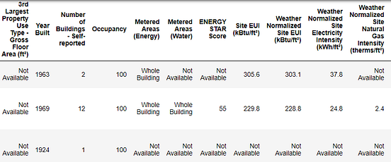 What Actual Data Looks Like!
This is a subset of the full data contains 60 columns.
Already, we can see a couple issues: first, we know that we want to predict the
What Actual Data Looks Like!
This is a subset of the full data contains 60 columns.
Already, we can see a couple issues: first, we know that we want to predict the  and decided to search for “Local Law 84”.
That led me to this page explains this is an NYC law requiring all buildings of a certain size to report their energy use.
More searching brought me to all the definitions of the columns. Maybe looking at a file name is an obvious place to start, but for me this was a reminder to go slow so you don’t miss anything important!
We don’t need to study all of the columns, but we should at least understand the Energy Star Score, is described as:
A 1-to-100 percentile ranking based on self-reported energy usage for the reporting year.
The Energy Star score is a relative measure used for comparing the energy efficiency of buildings.
That clears up the first problem, but the second issue is that missing values are encoded as “Not Available”.
This is a string in Python means that even the columns with numbers will be stored as
and decided to search for “Local Law 84”.
That led me to this page explains this is an NYC law requiring all buildings of a certain size to report their energy use.
More searching brought me to all the definitions of the columns. Maybe looking at a file name is an obvious place to start, but for me this was a reminder to go slow so you don’t miss anything important!
We don’t need to study all of the columns, but we should at least understand the Energy Star Score, is described as:
A 1-to-100 percentile ranking based on self-reported energy usage for the reporting year.
The Energy Star score is a relative measure used for comparing the energy efficiency of buildings.
That clears up the first problem, but the second issue is that missing values are encoded as “Not Available”.
This is a string in Python means that even the columns with numbers will be stored as 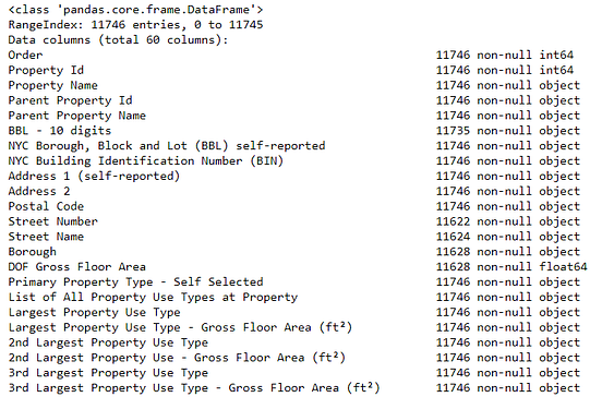 Sure enough, some of the columns that clearly contain numbers (such as ft²), are stored as objects.
We can’t do numerical analysis on strings, so these will have to be converted to number (specifically
Sure enough, some of the columns that clearly contain numbers (such as ft²), are stored as objects.
We can’t do numerical analysis on strings, so these will have to be converted to number (specifically 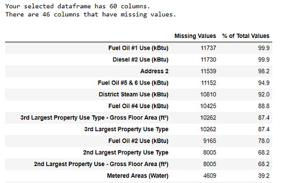 (To create this table, I used a function from this Stack Overflow Forum).
While we always want to be careful about removing information, if a column has a high percentage of missing values, then it probably will not be useful to our model.
The threshold for removing columns should depend on the problem (here is a discussion), and for this project, we will remove any columns with more than 50% missing values.
At this point, we may also want to remove outliers.
These can be due to typos in data entry, mistakes in units, or they could be legitimate but extreme values.
For this project, we will remove anomalies based on the definition of extreme outliers:
(To create this table, I used a function from this Stack Overflow Forum).
While we always want to be careful about removing information, if a column has a high percentage of missing values, then it probably will not be useful to our model.
The threshold for removing columns should depend on the problem (here is a discussion), and for this project, we will remove any columns with more than 50% missing values.
At this point, we may also want to remove outliers.
These can be due to typos in data entry, mistakes in units, or they could be legitimate but extreme values.
For this project, we will remove anomalies based on the definition of extreme outliers:
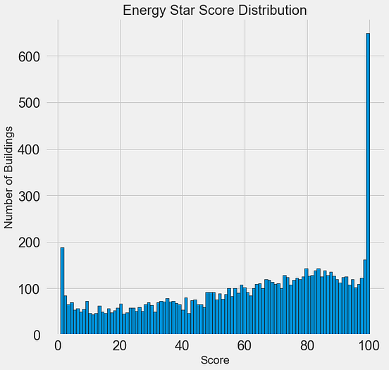 This looks quite suspicious! The Energy Star score is a percentile rank, means we would expect to see a uniform distribution, with each score assigned to the same number of buildings.
However, a disproportionate number of buildings have either the highest, 100, or the lowest, 1, score (higher is better for the Energy Star score).
If we go back to the definition of the score, we see that it is based on “self-reported energy usage” might explain the very high scores.
Asking building owners to report their own energy usage is like asking students to report their own scores on a test! As a result, this probably is not the most objective measure of a building’s energy efficiency.
If we had an unlimited amount of time, we might want to investigate why so many buildings have very high and very low scores we could by selecting these buildings and seeing what they have in common.
However, our objective is only to predict the score and not to devise a better method of scoring buildings! We can make a note in our report that the scores have a suspect distribution, but our main focus in on predicting the score.
This looks quite suspicious! The Energy Star score is a percentile rank, means we would expect to see a uniform distribution, with each score assigned to the same number of buildings.
However, a disproportionate number of buildings have either the highest, 100, or the lowest, 1, score (higher is better for the Energy Star score).
If we go back to the definition of the score, we see that it is based on “self-reported energy usage” might explain the very high scores.
Asking building owners to report their own energy usage is like asking students to report their own scores on a test! As a result, this probably is not the most objective measure of a building’s energy efficiency.
If we had an unlimited amount of time, we might want to investigate why so many buildings have very high and very low scores we could by selecting these buildings and seeing what they have in common.
However, our objective is only to predict the score and not to devise a better method of scoring buildings! We can make a note in our report that the scores have a suspect distribution, but our main focus in on predicting the score.
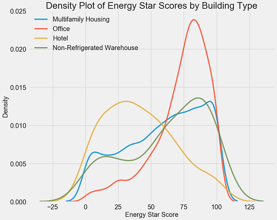 We can see that the building type has a significant impact on the Energy Star Score.
Office buildings tend to have a higher score while Hotels have a lower score.
This tells us that we should include the building type in our modeling because it does have an impact on the target.
As a categorical variable, we will have to one-hot encode the building type.
A similar plot can be used to show the Energy Star Score by borough:
We can see that the building type has a significant impact on the Energy Star Score.
Office buildings tend to have a higher score while Hotels have a lower score.
This tells us that we should include the building type in our modeling because it does have an impact on the target.
As a categorical variable, we will have to one-hot encode the building type.
A similar plot can be used to show the Energy Star Score by borough:
 The borough does not seem to have as large of an impact on the score as the building type.
Nonetheless, we might want to include it in our model because there are slight differences between the boroughs.
To quantify relationships between variables, we can use the Pearson Correlation Coefficient.
This is a measure of the strength and direction of a linear relationship between two variables.
A score of +1 is a perfectly linear positive relationship and a score of -1 is a perfectly negative linear relationship.
Several values of the correlation coefficient are shown below:
The borough does not seem to have as large of an impact on the score as the building type.
Nonetheless, we might want to include it in our model because there are slight differences between the boroughs.
To quantify relationships between variables, we can use the Pearson Correlation Coefficient.
This is a measure of the strength and direction of a linear relationship between two variables.
A score of +1 is a perfectly linear positive relationship and a score of -1 is a perfectly negative linear relationship.
Several values of the correlation coefficient are shown below:
 Values of the Pearson Correlation Coefficient (Source)
While the correlation coefficient cannot capture non-linear relationships, it is a good way to start figuring out how variables are related.
In Pandas, we can easily calculate the correlations between any columns in a dataframe:
# Find all correlations with the score and sort
correlations_data = data.corr()['score'].sort_values()
The most negative (left) and positive (right) correlations with the target:
Values of the Pearson Correlation Coefficient (Source)
While the correlation coefficient cannot capture non-linear relationships, it is a good way to start figuring out how variables are related.
In Pandas, we can easily calculate the correlations between any columns in a dataframe:
# Find all correlations with the score and sort
correlations_data = data.corr()['score'].sort_values()
The most negative (left) and positive (right) correlations with the target:

 There are several strong negative correlations between the features and the target with the most negative the different categories of EUI (these measures vary slightly in how they are calculated).
The EUI — Energy Use Intensity — is the amount of energy used by a building divided by the square footage of the buildings.
It is meant to be a measure of the efficiency of a building with a lower score being better.
Intuitively, these correlations make sense: as the EUI increases, the Energy Star Score tends to decrease.
There are several strong negative correlations between the features and the target with the most negative the different categories of EUI (these measures vary slightly in how they are calculated).
The EUI — Energy Use Intensity — is the amount of energy used by a building divided by the square footage of the buildings.
It is meant to be a measure of the efficiency of a building with a lower score being better.
Intuitively, these correlations make sense: as the EUI increases, the Energy Star Score tends to decrease.
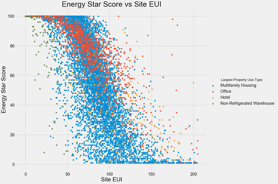 This plot lets us visualize what a correlation coefficient of -0.7 looks like.
As the Site EUI decreases, the Energy Star Score increases, a relationship that holds steady across the building types.
The final exploratory plot we will make is known as the Pairs Plot.
This is a great exploration tool because it lets us see relationships between multiple pairs of variables as well as distributions of single variables.
Here we are using the seaborn visualization library and the
This plot lets us visualize what a correlation coefficient of -0.7 looks like.
As the Site EUI decreases, the Energy Star Score increases, a relationship that holds steady across the building types.
The final exploratory plot we will make is known as the Pairs Plot.
This is a great exploration tool because it lets us see relationships between multiple pairs of variables as well as distributions of single variables.
Here we are using the seaborn visualization library and the 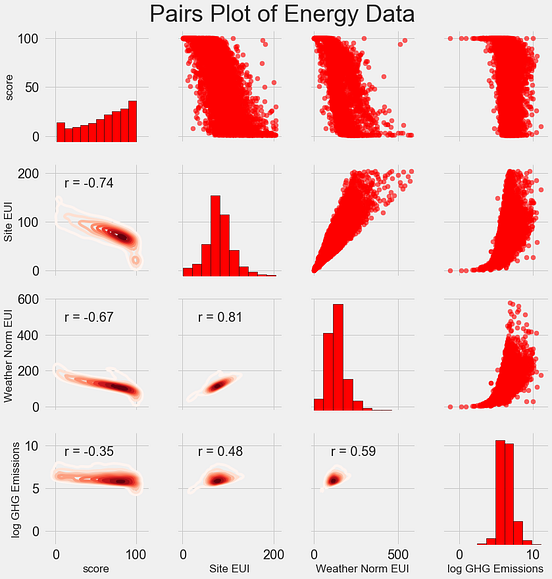 To see interactions between variables, we look for where a row intersects with a column.
For example, to see the correlation of
To see interactions between variables, we look for where a row intersects with a column.
For example, to see the correlation of 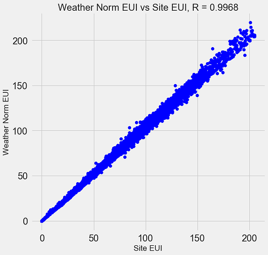 Features that are strongly correlated with each other are known as collinear and removing one of the variables in these pairs of features can often help a machine learning model generalize and be more interpretable.
(I should point out we are talking about correlations of features with other features, not correlations with the target, help our model!)
There are a number of methods to calculate collinearity between features, with one of the most common the variance inflation factor.
In this project, we will use thebcorrelation coefficient to identify and remove collinear features.
We will drop one of a pair of features if the correlation coefficient between them is greater than 0.6.
For the implementation, take a look at the notebook (and this Stack Overflow answer)
While this value may seem arbitrary, I tried several different thresholds, and this choice yielded the best model.
Machine learning is an empirical field and is often about experimenting and finding what performs best! After feature selection, we are left with 64 total features and 1 target.
# Remove any columns with all na values
features = features.dropna(axis=1, how = 'all')
print(features.shape)
(11319, 65)
Features that are strongly correlated with each other are known as collinear and removing one of the variables in these pairs of features can often help a machine learning model generalize and be more interpretable.
(I should point out we are talking about correlations of features with other features, not correlations with the target, help our model!)
There are a number of methods to calculate collinearity between features, with one of the most common the variance inflation factor.
In this project, we will use thebcorrelation coefficient to identify and remove collinear features.
We will drop one of a pair of features if the correlation coefficient between them is greater than 0.6.
For the implementation, take a look at the notebook (and this Stack Overflow answer)
While this value may seem arbitrary, I tried several different thresholds, and this choice yielded the best model.
Machine learning is an empirical field and is often about experimenting and finding what performs best! After feature selection, we are left with 64 total features and 1 target.
# Remove any columns with all na values
features = features.dropna(axis=1, how = 'all')
print(features.shape)
(11319, 65)
 Keras 自带一些样本数据集,如 MNIST 手写数字数据集。
以上代码可以加载这些数据,数据集图像是 NumPy 数组格式。
Keras 还做了一点图像预处理,使数据适用于模型。
Keras 自带一些样本数据集,如 MNIST 手写数字数据集。
以上代码可以加载这些数据,数据集图像是 NumPy 数组格式。
Keras 还做了一点图像预处理,使数据适用于模型。
 以上代码展示了模型。
在 Keras(TensorFlow)上,我们首先需要定义要使用的东西,然后立刻运行。
在 Keras 中,我们无法随时随地进行试验,不过 PyTorch 可以。
以上代码展示了模型。
在 Keras(TensorFlow)上,我们首先需要定义要使用的东西,然后立刻运行。
在 Keras 中,我们无法随时随地进行试验,不过 PyTorch 可以。
 以上的代码用于训练和评估模型。
我们可以使用 save() 函数来保存模型,以便后续用 load_model() 函数加载模型。
predict() 函数则用来获取模型在测试数据上的输出。
现在我们概览了 Keras 基本模型实现过程,现在来看 PyTorch。
PyTorch 中的模型实现研究人员大多使用 PyTorch,因为它比较灵活,代码样式也是试验性的。
你可以在 PyTorch 中调整任何事,并控制全部,但控制也伴随着责任。
在 PyTorch 里进行试验是很容易的。
因为你不需要先定义好每一件事再运行。
我们能够轻松测试每一步。
因此,在 PyTorch 中 debug 要比在 Keras 中容易一些。
接下来,我们来看简单的数字识别模型实现。
以上的代码用于训练和评估模型。
我们可以使用 save() 函数来保存模型,以便后续用 load_model() 函数加载模型。
predict() 函数则用来获取模型在测试数据上的输出。
现在我们概览了 Keras 基本模型实现过程,现在来看 PyTorch。
PyTorch 中的模型实现研究人员大多使用 PyTorch,因为它比较灵活,代码样式也是试验性的。
你可以在 PyTorch 中调整任何事,并控制全部,但控制也伴随着责任。
在 PyTorch 里进行试验是很容易的。
因为你不需要先定义好每一件事再运行。
我们能够轻松测试每一步。
因此,在 PyTorch 中 debug 要比在 Keras 中容易一些。
接下来,我们来看简单的数字识别模型实现。
 以上代码导入了必需的库,并定义了一些变量。
n_epochs、momentum 等变量都是必须设置的超参数。
此处不讨论细节,我们的目的是理解代码的结构。
以上代码导入了必需的库,并定义了一些变量。
n_epochs、momentum 等变量都是必须设置的超参数。
此处不讨论细节,我们的目的是理解代码的结构。
 以上代码旨在声明用于加载训练所用批量数据的数据加载器。
下载数据有很多种方式,不受框架限制。
如果你刚开始学习深度学习,以上代码可能看起来比较复杂。
以上代码旨在声明用于加载训练所用批量数据的数据加载器。
下载数据有很多种方式,不受框架限制。
如果你刚开始学习深度学习,以上代码可能看起来比较复杂。
 在此,我们定义了模型。
这是一种创建网络的通用方法。
我们扩展了 nn.Module,在前向传递中调用 forward() 函数。
PyTorch 的实现比较直接,且能够根据需要进行修改。
在此,我们定义了模型。
这是一种创建网络的通用方法。
我们扩展了 nn.Module,在前向传递中调用 forward() 函数。
PyTorch 的实现比较直接,且能够根据需要进行修改。

 以上代码段定义了训练和测试函数。
在 Keras 中,我们需要调用 fit() 函数把这些事自动做完。
但是在 PyTorch 中,我们必须手动执行这些步骤。
像 Fastai 这样的高级 API 库会简化它,训练所需的代码也更少。
以上代码段定义了训练和测试函数。
在 Keras 中,我们需要调用 fit() 函数把这些事自动做完。
但是在 PyTorch 中,我们必须手动执行这些步骤。
像 Fastai 这样的高级 API 库会简化它,训练所需的代码也更少。
 最后,保存和加载模型,以进行二次训练或预测。
这部分没有太多差别。
PyTorch 模型通常有 pt 或 pth 扩展。
关于框架选择的建议学会一种模型并理解其概念后,再转向另一种模型,并不是件难事,只是需要一些时间。
Colab 链接:PyTorch:https://colab.research.google.com/drive/1irYr0byhK6XZrImiY4nt9wX0fRp3c9mx?usp=sharing
Keras:https://colab.research.google.com/drive/1QH6VOY_uOqZ6wjxP0K8anBAXmI0AwQCm?usp=sharing
原文链接:https://medium.com/@karan_jakhar/keras-vs-pytorch-dilemma-dc434e5b5ae0
自动化数据增强:实践、理论和新方向
最后,保存和加载模型,以进行二次训练或预测。
这部分没有太多差别。
PyTorch 模型通常有 pt 或 pth 扩展。
关于框架选择的建议学会一种模型并理解其概念后,再转向另一种模型,并不是件难事,只是需要一些时间。
Colab 链接:PyTorch:https://colab.research.google.com/drive/1irYr0byhK6XZrImiY4nt9wX0fRp3c9mx?usp=sharing
Keras:https://colab.research.google.com/drive/1QH6VOY_uOqZ6wjxP0K8anBAXmI0AwQCm?usp=sharing
原文链接:https://medium.com/@karan_jakhar/keras-vs-pytorch-dilemma-dc434e5b5ae0
自动化数据增强:实践、理论和新方向
 另外MyQR还支持动态图片。
 当然这只是最简单的词云,词云更详细的操作可以参见WordCloud生成卡卡西忍术词云[1]。
 其中左边为原图,右边为抠图后填充黄色背景图。


 And finally, in SM one can do contour plots on linear and log scales, so I spent a little time trying to figure out how to do this in matplotlib.
Here is an example when the y points need to be plotted on the log scale and the x points still on the linear scale:
And finally, in SM one can do contour plots on linear and log scales, so I spent a little time trying to figure out how to do this in matplotlib.
Here is an example when the y points need to be plotted on the log scale and the x points still on the linear scale:

 Sometimes, a development machine will have Python 2 and Python 3 installed side by side.
Having two Python versions available is common on macOS.
If that is the case for you, you can use the python3 command to run Python 3 even if Python 2 is the default in your environment:
Sometimes, a development machine will have Python 2 and Python 3 installed side by side.
Having two Python versions available is common on macOS.
If that is the case for you, you can use the python3 command to run Python 3 even if Python 2 is the default in your environment:
 If you don’t have Python 3 installed yet, visit the Python Downloads page for instructions on installing it.
Launch a Python interpreter by running the python3 command in your shell:
If you don’t have Python 3 installed yet, visit the Python Downloads page for instructions on installing it.
Launch a Python interpreter by running the python3 command in your shell:

 Once you’ve installed the modules, use the import statement to make the modules available in your program:

 The help function uses the system text pagination program, also known as the pager, to display the documentation.
Many systems use less as the default text pager, just in case you aren’t familiar with the Vi shortcuts here are the basics:
The help function uses the system text pagination program, also known as the pager, to display the documentation.
Many systems use less as the default text pager, just in case you aren’t familiar with the Vi shortcuts here are the basics:

 There are many more useful string methods in Python, find out more about them in the Python string docs.
 Find all other Pandas data import functions in the Pandas docs.


 Once the model is set up we can use it to predict a result:
 For more details on the functionality available in Pandas, visit the Pandas user guides.
For more powerful math with NumPy (it can be used together with Pandas), check out the NumPy getting started guide.
For more details on the functionality available in Pandas, visit the Pandas user guides.
For more powerful math with NumPy (it can be used together with Pandas), check out the NumPy getting started guide.
 Gives (#rows, #columns)
给出行数和列数。
data.describe()
计算基本的统计数据。
Gives (#rows, #columns)
给出行数和列数。
data.describe()
计算基本的统计数据。
 .plot() 输出的示例data[ column_numerical ].hist()
画出数据分布(直方图)
.plot() 输出的示例data[ column_numerical ].hist()
画出数据分布(直方图)
 .hist() 输出的示例%matplotlib inline
如果你在使用 Jupyter,不要忘记在画图之前加上以上代码。
.hist() 输出的示例%matplotlib inline
如果你在使用 Jupyter,不要忘记在画图之前加上以上代码。
 image
.value_counts() 函数输出示例
image
.value_counts() 函数输出示例
 image
在 Jupyter 中使用 tqdm 和 pandas 得到的进度条
image
在 Jupyter 中使用 tqdm 和 pandas 得到的进度条
 image
.corr() 会给出相关性矩阵
pd.plotting.scatter_matrix(data, figsize=(12,8))
image
.corr() 会给出相关性矩阵
pd.plotting.scatter_matrix(data, figsize=(12,8))
 image
散点矩阵的例子。
它在同一幅图中画出了两列的所有组合。
image
散点矩阵的例子。
它在同一幅图中画出了两列的所有组合。
 image
正如前面解释过的,为了优化代码,在一行中将你的函数连接起来。
image
正如前面解释过的,为了优化代码,在一行中将你的函数连接起来。
 结语
remgb简单介绍就到这里了
结语
remgb简单介绍就到这里了

 In classic mode there is a server and a client.
The server advertises and the client connects.
With BLE there are different terms of peripheral and central.
A peripheral advertises and a central scans and connects.
In BLE you can also have a Broadcaster (beacon) which is a transmitter only
(connectionless) application.
The Observer (scanner) role is for receiver only connectionless applications.
In classic mode there is a server and a client.
The server advertises and the client connects.
With BLE there are different terms of peripheral and central.
A peripheral advertises and a central scans and connects.
In BLE you can also have a Broadcaster (beacon) which is a transmitter only
(connectionless) application.
The Observer (scanner) role is for receiver only connectionless applications.
 To get rid of the progress bars, probability table, and all the noise use the quiet mode.
 msg = "Do you want to continue?"
title = "Please Confirm"
if ccbox(msg, title): # show a Continue/Cancel dialog
pass # user chose Continue else: # user chose Cancel
sys.exit(0)
msg = "Do you want to continue?"
title = "Please Confirm"
if ccbox(msg, title): # show a Continue/Cancel dialog
pass # user chose Continue else: # user chose Cancel
sys.exit(0)
 Another example of a choicebox:
 In the multenterbox:
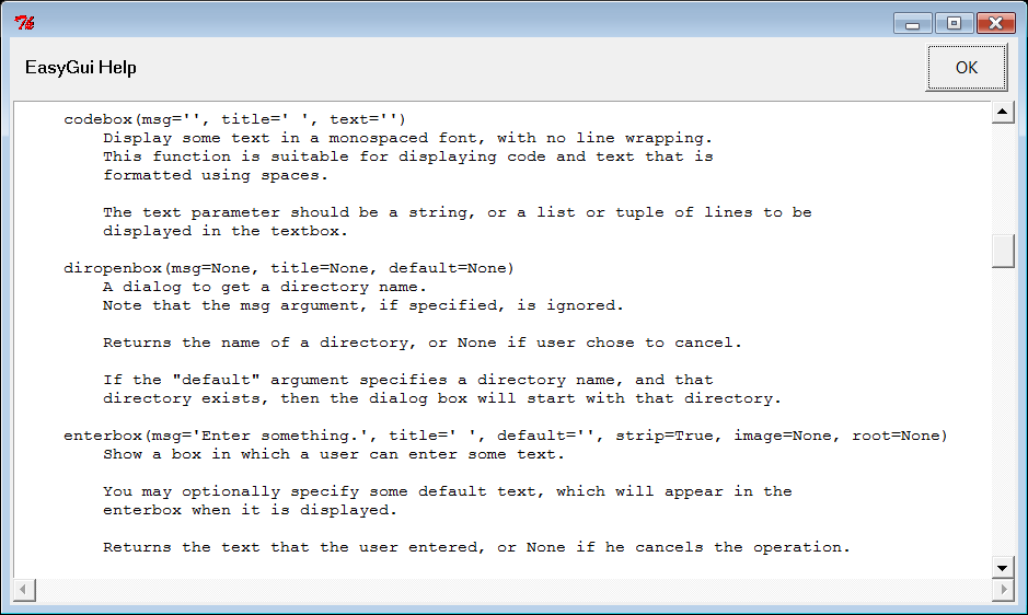 Note that you can pass codebox() and textbox() either a string or a list of strings. A list of strings will be converted to text before being displayed. This means that you can use these functions to display the contents of a file this way:
import os filename = os.path.normcase("c:/autoexec.bat")
f = open(filename, "r")
text = f.readlines()
f.close()
codebox("Contents of file " + filename, "Show File Contents", text)
Note that you can pass codebox() and textbox() either a string or a list of strings. A list of strings will be converted to text before being displayed. This means that you can use these functions to display the contents of a file this way:
import os filename = os.path.normcase("c:/autoexec.bat")
f = open(filename, "r")
text = f.readlines()
f.close()
codebox("Contents of file " + filename, "Show File Contents", text)
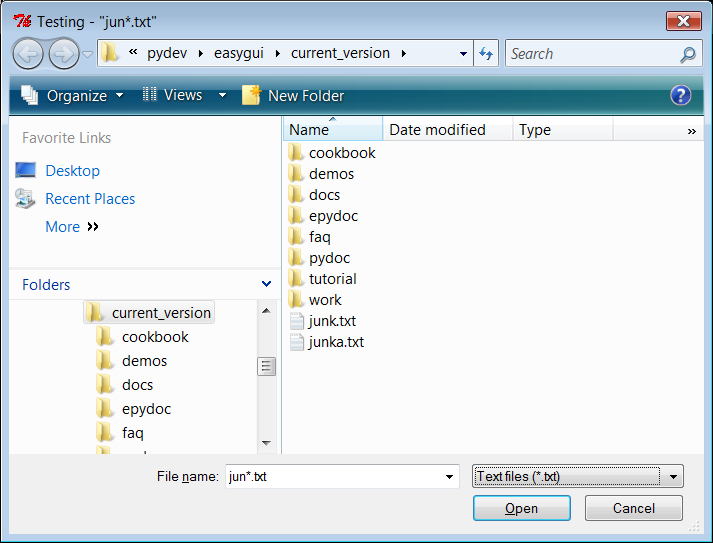
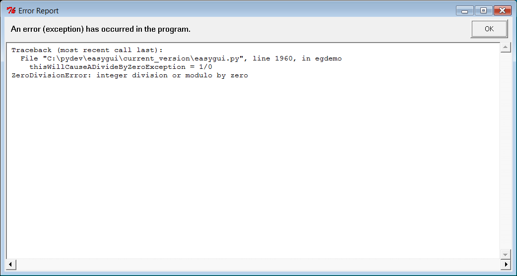
、Firefox、Safari(基于 WebKit) ,提供完善的自动化控制的 API。
Playwright 支持移动端页面测试,使用设备模拟技术可以使我们在移动 Web 浏览器中测试响应式 Web 应用程序。
Playwright 支持所有浏览器的 Headless 模式和非 Headless 模式的测试。
Playwright 的安装和配置非常简单,安装过程中会自动安装对应的浏览器和驱动,不需要额外配置 WebDriver 等。
Playwright 提供了自动等待相关的 API,当页面加载的时候会自动等待对应的节点加载,大大简化了 API 编写复杂度。
本节我们就来了解下 Playwright 的使用方法。
<h3>2. 安装</h3>Playwright 目前提供了 Python 和 Node.js 的 API,下面我们针对 Python 版的 Playwright 进行介绍。
要使用 Playwright,需要 Python 3.7 版本及以上,请确保 Python 的版本符合要求。
要安装 Playwright,可以直接使用 pip3,命令如下:
<code>
pip3 install playwright
</code>
安装完成之后需要进行一些初始化操作:
<code>
playwright install
</code>
这时候 Playwrigth 会安装 Chromium, Firefox and WebKit 浏览器并配置一些驱动,我们不必关心中间配置的过程,Playwright 会为我们配置好。
具体的安装说明可以参考:
https://setup.scrape.center/playwright。
安装完成之后,我们便可以使用 Playwright 启动 Chromium 或 Firefox 或 WebKit 浏览器来进行自动化操作了。
<h3>3. 基本使用</h3>Playwright 支持两种编写模式,一种是类似 Pyppetter 一样的异步模式,另一种是像 Selenium 一样的同步模式,我们可以根据实际需要选择使用不同的模式。
我们先来看一个基本同步模式的例子:
<code>
from playwright.sync_api import sync_playwright
with sync_playwright() as p:
for browser_type in [p.chromium, p.firefox, p.webkit]:
browser = browser_type.launch(headless=False)
page = browser.new_page()
page.goto('https://www.baidu.com')
page.screenshot(path=f'screenshot-{browser_type.name}.png')
print(page.title())
browser.close()
</code>
首先我们导入了 sync_playwright 方法,然后直接调用了这个方法,该方法返回的是一个 PlaywrightContextManager 对象,可以理解是一个浏览器上下文管理器,我们将其赋值为变量 p。
接着我们调用了 PlaywrightContextManager 对象的 chromium、firefox、webkit 属性依次创建了一个 Chromium、Firefox 以及 Webkit 浏览器实例,接着用一个 for 循环依次执行了它们的 launch 方法,同时设置了 headless 参数为 False。
“注意:
如果不设置为 False,默认是无头模式启动浏览器,我们看不到任何窗口。
”launch 方法返回的是一个 Browser 对象,我们将其赋值为 browser 变量。
然后调用 browser 的 new_page 方法,相当于新建了一个选项卡,返回的是一个 Page 对象,将其赋值为 page,这整个过程其实和 Pyppeteer 非常类似。
接着我们就可以调用 page 的一系列 API 来进行各种自动化操作了,比如调用 goto,就是加载某个页面,这里我们访问的是百度的首页。
接着我们调用了 page 的 screenshot 方法,参数传一个文件名称,这样截图就会自动保存为该图片名称,这里名称中我们加入了 browser_type 的 name 属性,代表浏览器的类型,结果分别就是 chromium, firefox, webkit。
另外我们还调用了 title 方法,该方法会返回页面的标题,即 HTML 中 title 节点中的文字,也就是选项卡上的文字,我们将该结果打印输出到控制台。
最后操作完毕,调用 browser 的 close 方法关闭整个浏览器,运行结束。
运行一下,这时候我们可以看到有三个浏览器依次启动并加载了百度这个页面,分别是 Chromium、Firefox 和 Webkit 三个浏览器,页面加载完成之后,生成截图、控制台打印结果就退出了。
这时候当前目录便会生成三个截图文件,都是百度的首页,文件名中都带有了浏览器的名称,如图所示:
<img src=) 控制台运行结果如下:
控制台运行结果如下:
:
if '/api/movie/' in response.url and response.status == 200:
print(response.json())
with sync_playwright() as p:
browser = p.chromium.launch(headless=False)
page = browser.new_page()
page.on('response', on_response)
page.goto('https://spa6.scrape.center/')
page.wait_for_load_state('networkidle')
browser.close()
</code>
控制台输入如下:
<code>
{'count': 100, 'results': [{'id': 1, 'name': '霸王别姬', 'alias': 'Farewell My Concubine', 'cover': 'https://p0.meituan.net/movie/ce4da3e03e655b5b88ed31b5cd7896cf62472.jpg@464w_644h_1e_1c', 'categories': ['剧情', '爱情'], 'published_at': '1993-07-26', 'minute': 171, 'score': 9.5, 'regions': ['中国大陆', '中国香港']},
...
'published_at': None, 'minute': 103, 'score': 9.0, 'regions': ['美国']}, {'id': 10, 'name': '狮子王', 'alias': 'The Lion King', 'cover': 'https://p0.meituan.net/movie/27b76fe6cf3903f3d74963f70786001e1438406.jpg@464w_644h_1e_1c', 'categories': ['动画', '歌舞', '冒险'], 'published_at': '1995-07-15', 'minute': 89, 'score': 9.0, 'regions': ['美国']}]}
</code>
简直是得来全不费工夫,我们直接通过这个方法拦截了 Ajax 请求,直接把响应结果拿到了,即使这个 Ajax 请求有加密参数,我们也不用关心,因为我们直接截获了 Ajax 最后响应的结果,这对数据爬取来说实在是太方便了。
另外还有很多其他的事件监听,这里不再一一介绍了,可以查阅官方文档,参考类似的写法实现。
<h3>获取页面源码</h3>要获取页面的 HTML 代码其实很简单,我们直接通过 content 方法获取即可,用法如下:
<code>
from playwright.sync_api import sync_playwright
with sync_playwright() as p:
browser = p.chromium.launch(headless=False)
page = browser.new_page()
page.goto('https://spa6.scrape.center/')
page.wait_for_load_state('networkidle')
html = page.content()
print(html)
browser.close()
</code>
运行结果就是页面的 HTML 代码。
获取了 HTML 代码之后,我们通过一些解析工具就可以提取想要的信息了。
<h3>页面点击</h3>刚才我们通过示例也了解了页面点击的方法,那就是 click,这里详细说一下其使用方法。
页面点击的 API 定义如下:
<code>
page.click(selector, **kwargs)
</code>
这里可以看到必传的参数是 selector,其他的参数都是可选的。
第一个 selector 就代表选择器,可以用来匹配想要点击的节点,如果传入的选择器匹配了多个节点,那么只会用第一个节点。
这个方法的内部执行逻辑如下:
根据 selector 找到匹配的节点,如果没有找到,那就一直等待直到超时,超时时间可以由额外的 timeout 参数设置,默认是 30 秒。
等待对该节点的可操作性检查的结果,比如说如果某个按钮设置了不可点击,那它会等待该按钮变成了可点击的时候才去点击,除非通过 force 参数设置跳过可操作性检查步骤强制点击。
如果需要的话,就滚动下页面,将需要被点击的节点呈现出来。
调用 page 对象的 mouse 方法,点击节点中心的位置,如果指定了 position 参数,那就点击指定的位置。
click 方法的一些比较重要的参数如下:
click_count:
点击次数,默认为 1。
timeout:
等待要点击的节点的超时时间,默认是 30 秒。
position:
需要传入一个字典,带有 x 和 y 属性,代表点击位置相对节点左上角的偏移位置。
force:
即使不可点击,那也强制点击。
默认是 False。
具体的 API 设置参数可以参考官方文档:
https://playwright.dev/python/docs/api/class-page/#pageclickselector-kwargs。
<h3>文本输入</h3>文本输入对应的方法是 fill,API 定义如下:
<code>
page.fill(selector, value, **kwargs)
</code>
这个方法有两个必传参数,第一个参数也是 selector,第二个参数是 value,代表输入的内容,另外还可以通过 timeout 参数指定对应节点的最长等待时间。
<h3>获取节点属性</h3>除了对节点进行操作,我们还可以获取节点的属性,方法就是 get_attribute,API 定义如下:
<code>
page.get_attribute(selector, name, **kwargs)
</code>
这个方法有两个必传参数,第一个参数也是 selector,第二个参数是 name,代表要获取的属性名称,另外还可以通过 timeout 参数指定对应节点的最长等待时间。
示例如下:
<code>
from playwright.sync_api import sync_playwright
with sync_playwright() as p:
browser = p.chromium.launch(headless=False)
page = browser.new_page()
page.goto('https://spa6.scrape.center/')
page.wait_for_load_state('networkidle')
href = page.get_attribute('a.name', 'href')
print(href)
browser.close()
</code>
这里我们调用了 get_attribute 方法,传入的 selector 是<code>a.name</code>,选定了 class 为 name 的 a 节点,然后第二个参数传入了 href,获取超链接的内容,输出结果如下:
<code>
/detail/ZWYzNCN0ZXVxMGJ0dWEjKC01N3cxcTVvNS0takA5OHh5Z2ltbHlmeHMqLSFpLTAtbWIx
</code>
可以看到对应 href 属性就获取出来了,但这里只有一条结果,因为这里有个条件,那就是如果传入的选择器匹配了多个节点,那么只会用第一个节点。
那怎么获取所有的节点呢?
<h3>获取多个节点</h3>获取所有节点可以使用 query_selector_all 方法,它可以返回节点列表,通过遍历获取到单个节点之后,我们可以接着调用单个节点的方法来进行一些操作和属性获取,示例如下:
<code>
from playwright.sync_api import sync_playwright
with sync_playwright() as p:
browser = p.chromium.launch(headless=False)
page = browser.new_page()
page.goto('https://spa6.scrape.center/')
page.wait_for_load_state('networkidle')
elements = page.query_selector_all('a.name')
for element in elements:
print(element.get_attribute('href'))
print(element.text_content())
browser.close()
</code>
这里我们通过 query_selector_all 方法获取了所有匹配到的节点,每个节点对应的是一个 ElementHandle 对象,然后 ElementHandle 对象也有 get_attribute 方法来获取节点属性,另外还可以通过 text_content 方法获取节点文本。
运行结果如下:
<code>
/detail/ZWYzNCN0ZXVxMGJ0dWEjKC01N3cxcTVvNS0takA5OHh5Z2ltbHlmeHMqLSFpLTAtbWIx
霸王别姬 - Farewell My Concubine
/detail/ZWYzNCN0ZXVxMGJ0dWEjKC01N3cxcTVvNS0takA5OHh5Z2ltbHlmeHMqLSFpLTAtbWIy
这个杀手不太冷 - Léon
/detail/ZWYzNCN0ZXVxMGJ0dWEjKC01N3cxcTVvNS0takA5OHh5Z2ltbHlmeHMqLSFpLTAtbWIz
肖申克的救赎 - The Shawshank Redemption
/detail/ZWYzNCN0ZXVxMGJ0dWEjKC01N3cxcTVvNS0takA5OHh5Z2ltbHlmeHMqLSFpLTAtbWI0
泰坦尼克号 - Titanic
/detail/ZWYzNCN0ZXVxMGJ0dWEjKC01N3cxcTVvNS0takA5OHh5Z2ltbHlmeHMqLSFpLTAtbWI1
罗马假日 - Roman Holiday
/detail/ZWYzNCN0ZXVxMGJ0dWEjKC01N3cxcTVvNS0takA5OHh5Z2ltbHlmeHMqLSFpLTAtbWI2
唐伯虎点秋香 - Flirting Scholar
/detail/ZWYzNCN0ZXVxMGJ0dWEjKC01N3cxcTVvNS0takA5OHh5Z2ltbHlmeHMqLSFpLTAtbWI3
乱世佳人 - Gone with the Wind
/detail/ZWYzNCN0ZXVxMGJ0dWEjKC01N3cxcTVvNS0takA5OHh5Z2ltbHlmeHMqLSFpLTAtbWI4
喜剧之王 - The King of Comedy
/detail/ZWYzNCN0ZXVxMGJ0dWEjKC01N3cxcTVvNS0takA5OHh5Z2ltbHlmeHMqLSFpLTAtbWI5
楚门的世界 - The Truman Show
/detail/ZWYzNCN0ZXVxMGJ0dWEjKC01N3cxcTVvNS0takA5OHh5Z2ltbHlmeHMqLSFpLTAtbWIxMA==
狮子王 - The Lion King
</code>
<h3>获取单个节点</h3>获取单个节点也有特定的方法,就是 query_selector,如果传入的选择器匹配到多个节点,那它只会返回第一个节点,示例如下:
<code>
from playwright.sync_api import sync_playwright
with sync_playwright() as p:
browser = p.chromium.launch(headless=False)
page = browser.new_page()
page.goto('https://spa6.scrape.center/')
page.wait_for_load_state('networkidle')
element = page.query_selector('a.name')
print(element.get_attribute('href'))
print(element.text_content())
browser.close()
</code>
运行结果如下:
<code>
/detail/ZWYzNCN0ZXVxMGJ0dWEjKC01N3cxcTVvNS0takA5OHh5Z2ltbHlmeHMqLSFpLTAtbWIx
霸王别姬 - Farewell My Concubine
</code>
可以看到这里只输出了第一个匹配节点的信息。
<h3>网络劫持</h3>最后再介绍一个实用的方法 route,利用 route 方法,我们可以实现一些网络劫持和修改操作,比如修改 request 的属性,修改 response 响应结果等。
看一个实例:
<code>
from playwright.sync_api import sync_playwright
import re
with sync_playwright() as p:
browser = p.chromium.launch(headless=False)
page = browser.new_page()
def cancel_request(route, request):
route.abort()
page.route(re.compile(r) 这里我们调用了 route 方法,第一个参数通过正则表达式传入了匹配的 URL 路径,这里代表的是任何包含
这里我们调用了 route 方法,第一个参数通过正则表达式传入了匹配的 URL 路径,这里代表的是任何包含 The page for JavaScript GitHub Topic
We will use Playwright to start a browser, open the GitHub topic page, click the Load more button to display more repositories, and then extract the following information:
Owner
Name
URL
Number of stars
Description
List of repository topics
The page for JavaScript GitHub Topic
We will use Playwright to start a browser, open the GitHub topic page, click the Load more button to display more repositories, and then extract the following information:
Owner
Name
URL
Number of stars
Description
List of repository topics
 JavaScript GitHub topic
 There are two things we need to tell Playwright to load more repositories:
Click the Load more… button.
Wait for the repositories to load.
Clicking buttons is extremely easy with Playwright.
By prefixing
There are two things we need to tell Playwright to load more repositories:
Click the Load more… button.
Wait for the repositories to load.
Clicking buttons is extremely easy with Playwright.
By prefixing 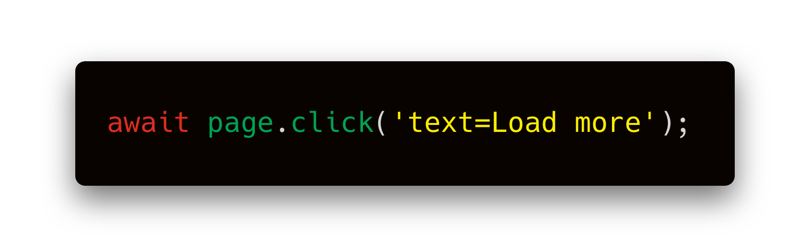 Clicking a button
This is a huge improvement over Puppeteer and it makes Playwright lovely to work with.
After clicking, we need to wait for the repositories to load.
If we didn’t, the scraper could finish before the new repositories show up on the page and we would miss that data.
Clicking a button
This is a huge improvement over Puppeteer and it makes Playwright lovely to work with.
After clicking, we need to wait for the repositories to load.
If we didn’t, the scraper could finish before the new repositories show up on the page and we would miss that data.
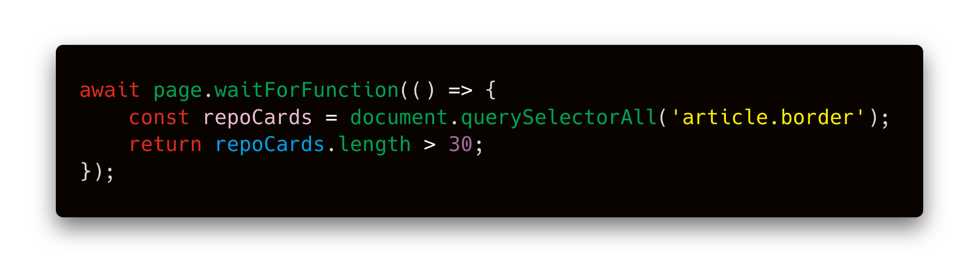 Waiting for
To find that
Waiting for
To find that 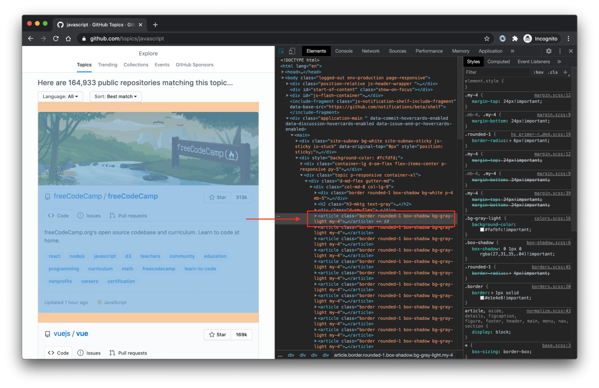 Chrome Dev Tools
Let’s plug this into our code and do a test run.
If you watch the run, you’ll see that the browser first scrolls down and clicks the Load more… button, which changes the text into Loading more.
After a second or two, you’ll see the next batch of 30 repositories appear.
Great job!
Chrome Dev Tools
Let’s plug this into our code and do a test run.
If you watch the run, you’ll see that the browser first scrolls down and clicks the Load more… button, which changes the text into Loading more.
After a second or two, you’ll see the next batch of 30 repositories appear.
Great job!
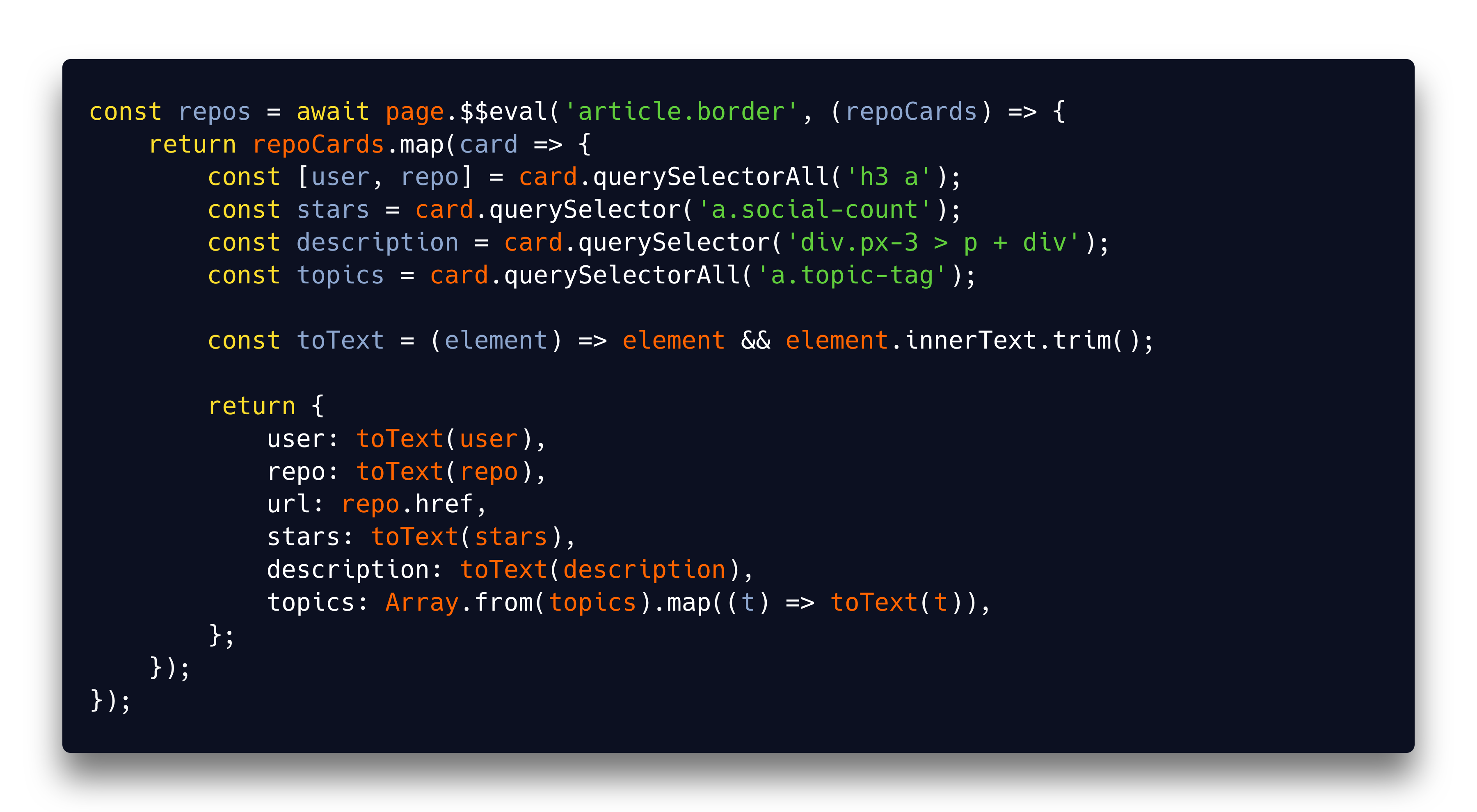 Extracting data from page
It works like this:
Extracting data from page
It works like this:  Result — Image By Author

Cleaning Download Folder
One of the messiest things in this world is the download folder of a developer. When writing a blog, working on a project, something similar we just download images and save them with ugly and funny names like asdfg.jpg. This python script will clean your download folder by renaming and deleting certain files based on some condition. Libraries:- OS import os folder_location = 'C:\\Users\\user\\Downloads\\demo' os.chdir(folder_location) list_of_files = os.listdir() ## Selecting All Images images = [content for content in list_of_files if content.endswith(('.png','.jpg','.jpeg'))] for index, image in enumerate(images): os.rename(image,f'{index}.png') ## Deleting All Images ################## Write Your Script Here ######## Try To Create Your Own CodeSending Text Messages
There are many free text message services available on the internet like Twillo, fast2sms, etc. Fast2sms provide 50 free messages with a prebuild template to connect your script with their API. This script will let us send text SMS to any number directly through our command-line interface. import requests import json def send_sms(number, message): url = 'https://www.fast2sms.com/dev/bulk' params = { 'authorization': 'FIND_YOUR_OWN', 'sender_id': 'FSTSMS', 'message': message, 'language': 'english', 'route': 'p', 'numbers': number } response = requests.get(url, params=params) dic = response.json() #print(dic) return dic.get('return') num = int(input("Enter The Number:\n")) msg = input("Enter The Message You Want To Send:\n") s = send_sms(num, msg) if s: print("Successfully sent") else: print("Something went wrong..")Converting hours to seconds
When working on projects that require you to convert hours into seconds, you can use the following Python script.def convert(seconds):
seconds = seconds % (24 * 3600)
hour = seconds // 3600
seconds %= 3600
minutes = seconds // 60
seconds %= 60
return "%d:%02d:%02d" % (hour, minutes, seconds)
# Driver program
n = 12345
print(convert(n))
Raising a number to the power
Another popular Python script calculates the power of a number. For example, 2 to the power of 4. Here, there are at least three methods to choose from. You can use the math.pow(), pow(), or **. Here is the script.import math
# Assign values to x and n
x = 4
n = 3
# Method 1
power = x ** n
print("%d to the power %d is %d" % (x,n,power))
# Method 2
power = pow(x,n)
print("%d to the power %d is %d" % (x,n,power))
# Method 3
power = math.pow(2,6.5)
print("%d to the power %d is %5.2f" % (x,n,power))
If/else statement
This is arguably one of the most used statements in Python. It allows your code to execute a function if a certain condition is met. Unlike other languages, you don’t need to use curly braces. Here is a simple if/else script.# Assign a value
number = 50
# Check the is more than 50 or not
if (number >= 50):
print("You have passed")
else:
print("You have not passed")
Convert images to JPEG
The most conventional systems rarely accept image formats such as PNG. As such, you’ll be required to convert them into JPEG files. Luckily, there’s a Python script that allows you to automate this process.import os
import sys
from PIL import Image
if len(sys.argv) > 1:
if os.path.exists(sys.argv[1]):
im = Image.open(sys.argv[1])
target_name = sys.argv[1] + ".jpg"
rgb_im = im.convert('RGB')
rgb_im.save(target_name)
print("Saved as " + target_name)
else:
print(sys.argv[1] + " not found")
else:
print("Usage: convert2jpg.py <file>")
Download Google images
If you are working on a project that demands many images, there’s a Python script that enables you to do so. With it, you can download hundreds of images simultaneously. However, you should avoid violating copyright terms. Click here for more information.Read battery level of Bluetooth device
This script allows you to read the battery level of your Bluetooth headset. This is especially crucial if the level does not display on your PC. However, it does not support all Bluetooth headsets. For it to run, you need to have Docker on your system. Click here for more information.Delete Telegram messages
Let’s face it, messaging apps do chew up much of your device’s storage space. And Telegram is no different. Luckily, this script allows you to delete all supergroups messages. You need to enter the supergroup’s information for the script to run. Click here for more information.Get song lyrics
This is yet another popular Python script that enables you to scrape lyrics from the Genius site. It primarily works with Spotify, however, other media players with DBus MediaPlayer2 can also use the script. With it, you can sing along to your favorite song. Click here for more information.Heroku hosting
Heroku is one of the most preferred hosting services. Used by thousands of developers, it allows you to build apps for free. Likewise, you can host your Python applications and scripts on Heroku with this script. Click here for more information.Github activity
If you contribute to open source projects, keeping a record of your contributions is recommended. Not only do you track your contributions, but also appear professional when displaying your work to other people. With this script, you can generate a robust activity graph. Click here for information.Removing duplicate code
When creating large apps or working on projects, it is normal to have duplicates in your list. This not only makes coding strenuous, but also makes your code appear unprofessional. With this script, you can remove duplicates seamlessly.Sending emails
Emails are crucial to any businesses’ communication avenues. With Python, you can enable sites and web apps to send them without hiccups. However, businesses do not want to send each email manually, instead, they prefer to automate the process. This script allows you to choose which emails to reply to.Find specific files on your system
Often, you forget the names or location of files on your system. This is not only annoying but also consumes time navigating through different folders. While there are programs that help you search for files, you need one that can automate the process. Luckily, this script enables you to choose which files and file types to search for. For example, if want to search for MP3 files, you can use this script.import fnmatch
import os
rootPath = '/'
pattern = '*.mp3'
for root, dirs, files in os.walk(rootPath):
for filename in fnmatch.filter(files, pattern):
print( os.path.join(root, filename))
Generating random passwords
Passwords bolster the privacy of app and website users. Besides, they prevent fraudulent use of accounts by cyber criminals. As such, you need to create an app or website that can generate random strong passwords. With this script, you can seamlessly generate them.import string
from random import *
characters = string.ascii_letters + string.punctuation + string.digits
password = "".join(choice(characters) for x in range(randint(8, 16)))
print (password)
Print odd numbers
Some projects may require you to print odd numbers within a specific range. While you can do this manually, it is time-consuming and prone to error. This means you need a program that can automate the process. Thanks to this script, you can achieve this.Get date value
Python allows you to format a date value in numerous ways. With the DateTime module, this script allows you to read the current date and set a custom value.Removing items from a list
You’ll often have to modify lists on your projects. Python enables you to do this using the Insert() and remove() methods. Here is a script you can use to achieve this.# Declare a fruit list
fruits = ["Mango","Orange","Guava","Banana"]
# Insert an item in the 2nd position
fruits.insert(1, "Grape")
# Displaying list after inserting
print("The fruit list after insert:")
print(fruits)
# Remove an item
fruits.remove("Guava")
# Print the list after delete
print("The fruit list after delete:")
print(fruits)
Count list items
Using the count() method, you can print how many times a string appears in another string. You need to provide the string that Python will search. Here is a script to help you do so.# Define the string
string = 'Python Bash Java PHP PHP PERL'
# Define the search string
search = 'P'
# Store the count value
count = string.count(search)
# Print the formatted output
print("%s appears %d times" % (search, count))
Text grabber
With this Python script, you can take a screenshot and copy the text in it. Click here for more information.Tweet search
Ever searched for a tweet to no avail? Annoying, right! Well, why not use this script and let it do the legwork for you.反爬虫代码 直接炸了爬虫服务器
很多人的爬虫是使用Requests来写的,如果你阅读过Requests的文档,那么你可能在文档中的Binary Response Content[1]这一小节,看到这样一句话: The gzip and deflate transfer-encodings are automatically decoded for you. (Request)会自动为你把gzip和deflate转码后的数据进行解码网站服务器可能会使用gzip压缩一些大资源,这些资源在网络上传输的时候,是压缩后的二进制格式。 客户端收到返回以后,如果发现返回的Headers里面有一个字段叫做Content-Encoding,其中的值包含gzip,那么客户端就会先使用gzip对数据进行解压,解压完成以后再把它呈现到客户端上面。
浏览器自动就会做这个事情,用户是感知不到这个事情发生的。
而requests、Scrapy这种网络请求库或者爬虫框架,也会帮你做这个事情,因此你不需要手动对网站返回的数据解压缩。
这个功能原本是一个方便开发者的功能,但我们可以利用这个功能来做报复爬虫的事情。
我们首先写一个客户端,来测试一下返回gzip压缩数据的方法。
我首先在硬盘上创建一个文本文件text.txt,里面有两行内容,如下图所示:
.gz文件:
cattext.txt|gzip>data.gz
接下来,我们使用FastAPI写一个HTTP服务器server.py:
from fastapi import FastAPI, Response
from fastapi.responses import FileResponse

app = FastAPI()
@app.get('/')

def index():
    resp = FileResponse('data.gz')
    return resp
然后使用命令uvicorn server:app启动这个服务。
接下来,我们使用requests来请求这个接口,会发现返回的数据是乱码,如下图所示:
server.py的代码,通过Headers告诉客户端,这个数据是经过gzip压缩的:
from fastapi import FastAPI, Response
from fastapi.responses import FileResponse

app = FastAPI()

@app.get('/')
def index():
    resp = FileResponse('data.gz')
    resp.headers['Content-Encoding'] = 'gzip'  # 说明这是gzip压缩的数据
    return resp
修改以后,重新启动服务器,再次使用requests请求,发现已经可以正常显示数据了:
111111111111111111111111111111111111111111111111111111111111111111111111111111111111111111111111111111111111111111111111111111111111111111111111111111111111111111111111111111111111111111111111我们可以用5个字符来表示:
192个1。
这就相当于把192个字符压缩成了5个字符,压缩率高达97.4%。
如果我们可以把一个1GB的文件压缩成1MB,那么对服务器来说,仅仅是返回了1MB的二进制数据,不会造成任何影响。
但是对客户端或者爬虫来说,它拿到这个1MB的数据以后,就会在内存中把它还原成1GB的内容。
这样一瞬间爬虫占用的内存就增大了1GB。
如果我们再进一步增大这个原始数据,那么很容易就可以把爬虫所在的服务器内存全部沾满,轻者服务器直接杀死爬虫进程,重则爬虫服务器直接死机。
你别以为这个压缩比听起来很夸张,其实我们使用很简单的一行命令就可以生成这样的压缩文件。
如果你用的是Linux,那么请执行命令:
dd if=/dev/zero bs=1M count=1000 | gzip > boom.gz
如果你的电脑是macOS,那么请执行命令:
dd if=/dev/zero bs=1048576 count=1000 | gzip > boom.gz
执行过程如下图所示:
boom.gz文件只有995KB。
但是如果我们使用gzip -d boom.gz对这个文件解压缩,就会发现生成了一个1GB的boom文件,如下图所示:
count=1000改成一个更大的数字,就能得到更大的文件。
我现在把count改成10,给大家做一个演示(不敢用1GB的数据来做测试,害怕我的Jupyter崩溃)。
生成的boom.gz文件只有10KB:
resp这个对象占用的内存大小:
Fancier Output Formatting
https://docs.python.org/3/tutorial/ So far we’ve encountered two ways of writing values: expression statements and theprint() function.
(A third way is using the write() method of file objects; the standard output file can be referenced as sys.stdout.
See the Library Reference for more information on this.)
Often you’ll want more control over the formatting of your output than simply printing space-separated values.
There are several ways to format output.
To use formatted string literals, begin a string with f or F before the opening quotation mark or triple quotation mark.
Inside this string, you can write a Python expression between { and }
characters that can refer to variables or literal values.
>>> year = 2016
>>> event = "Referendum"
>>> f"Results of the {year} {event}"
"Results of the 2016 Referendum"
The str.format() method of strings requires more manual effort.
You’ll still use { and } to mark where a variable will be substituted and can provide detailed formatting directives,
but you’ll also need to provide the information to be formatted.
>>> yes_votes = 42_572_654
>>> no_votes = 43_132_495
>>> percentage = yes_votes / (yes_votes + no_votes)
>>> "{:-9} YES votes {:2.2%}".format(yes_votes, percentage)
" 42572654 YES votes 49.67%"
Finally, you can do all the string handling yourself by using string slicing and concatenation operations to create any layout you can imagine.
The string type has some methods that perform useful operations for padding strings to a given column width.
When you don’t need fancy output but just want a quick display of some variables for debugging purposes, you can convert any value to a string with the repr() or str() functions.
The str() function is meant to return representations of values which are fairly human-readable, while repr() is meant to generate representations which can be read by the interpreter (or will force a SyntaxError if there is no equivalent syntax).
For objects which don’t have a particular representation for human consumption, str() will return the same value as
repr().
Many values, such as numbers or structures like lists and dictionaries, have the same representation using either function.
Strings, in particular, have two distinct representations.
Some examples:
>>> s = "Hello, world."
>>> str(s)
"Hello, world."
>>> repr(s)
""Hello, world.""
>>> str(1/7)
"0.14285714285714285"
>>> x = 10 * 3.25
>>> y = 200 * 200
>>> s = "The value of x is " + repr(x) + ", and y is " + repr(y) + "..."
>>> print(s)
The value of x is 32.5, and y is 40000...
>>> # The repr() of a string adds string quotes and backslashes:
...
hello = "hello, world\n"
>>> hellos = repr(hello)
>>> print(hellos)
"hello, world\n"
>>> # The argument to repr() may be any Python object:
...
repr((x, y, ("spam", "eggs")))
"(32.5, 40000, ("spam", "eggs"))"
The string module contains a Template class that offers yet another way to substitute values into strings, using placeholders like
$x and replacing them with values from a dictionary, but offers much less control of the formatting.
7.1.1. Formatted String Literals
Formatted string literals (also called f-strings for short) let you include the value of Python expressions inside a string by prefixing the string with f or F and writing expressions as
{expression}.
An optional format specifier can follow the expression.
This allows greater control over how the value is formatted.
The following example rounds pi to three places after the decimal:
>>> import math
>>> print(f"The value of pi is approximately {math.pi:.3f}.")
The value of pi is approximately 3.142.
Passing an integer after the ':' will cause that field to be a minimum number of characters wide.
This is useful for making columns line up.
>>> table = {"Sjoerd": 4127, "Jack": 4098, "Dcab": 7678}
>>> for name, phone in table.items():
...
print(f"{name:10} ==> {phone:10d}")
...
Sjoerd ==> 4127
Jack ==> 4098
Dcab ==> 7678
Other modifiers can be used to convert the value before it is formatted.
'!a' applies ascii(), '!s' applies str(), and '!r'
applies repr():
>>> animals = "eels"
>>> print(f"My hovercraft is full of {animals}.")
My hovercraft is full of eels.
>>> print(f"My hovercraft is full of {animals!r}.")
My hovercraft is full of "eels".
The = specifier can be used to expand an expression to the text of the expression, an equal sign, then the representation of the evaluated expression:
>>> bugs = "roaches"
>>> count = 13
>>> area = "living room"
>>> print(f"Debugging {bugs=} {count=} {area=}")
Debugging bugs="roaches" count=13 area="living room"
See self-documenting expressions for more information on the = specifier.
For a reference on these format specifications, see the reference guide for the Format Specification Mini-Language.
7.1.2. The String format() Method
Basic usage of the str.format() method looks like this:
>>> print("We are the {} who say "{}!"".format("knights", "Ni"))
We are the knights who say "Ni!"
The brackets and characters within them (called format fields) are replaced with the objects passed into the str.format() method.
A number in the brackets can be used to refer to the position of the object passed into the
str.format() method.
>>> print("{0} and {1}".format("spam", "eggs"))
spam and eggs
>>> print("{1} and {0}".format("spam", "eggs"))
eggs and spam If keyword arguments are used in the str.format() method, their values are referred to by using the name of the argument.
>>> print("This {food} is {adjective}.".format(
...
food="spam", adjective="absolutely horrible"))
This spam is absolutely horrible.
Positional and keyword arguments can be arbitrarily combined:
>>> print("The story of {0}, {1}, and {other}.".format("Bill", "Manfred",
...
other="Georg"))
The story of Bill, Manfred, and Georg.
If you have a really long format string that you don’t want to split up, it would be nice if you could reference the variables to be formatted by name instead of by position.
This can be done by simply passing the dict and using square brackets '[]' to access the keys.
>>> table = {"Sjoerd": 4127, "Jack": 4098, "Dcab": 8637678}
>>> print("Jack: {0[Jack]:d}; Sjoerd: {0[Sjoerd]:d}; "
...
"Dcab: {0[Dcab]:d}".format(table))
Jack: 4098; Sjoerd: 4127; Dcab: 8637678
This could also be done by passing the table dictionary as keyword arguments with the **
notation.
>>> table = {"Sjoerd": 4127, "Jack": 4098, "Dcab": 8637678}
>>> print("Jack: {Jack:d}; Sjoerd: {Sjoerd:d}; Dcab: {Dcab:d}".format(**table))
Jack: 4098; Sjoerd: 4127; Dcab: 8637678
This is particularly useful in combination with the built-in function
vars(), which returns a dictionary containing all local variables.
As an example, the following lines produce a tidily aligned set of columns giving integers and their squares and cubes:
>>> for x in range(1, 11):
...
print("{0:2d} {1:3d} {2:4d}".format(x, x*x, x*x*x))
...
1 1 1
2 4 8
3 9 27
4 16 64
5 25 125
6 36 216
7 49 343
8 64 512
9 81 729
10 100 1000
For a complete overview of string formatting with str.format(), see Format String Syntax.
7.1.3. Manual String Formatting
Here’s the same table of squares and cubes, formatted manually:
>>> for x in range(1, 11):
...
print(repr(x).rjust(2), repr(x*x).rjust(3), end=" ")
...
# Note use of "end" on previous line
...
print(repr(x*x*x).rjust(4))
...
1 1 1
2 4 8
3 9 27
4 16 64
5 25 125
6 36 216
7 49 343
8 64 512
9 81 729
10 100 1000
(Note that the one space between each column was added by the way print() works: it always adds spaces between its arguments.)
The str.rjust() method of string objects right-justifies a string in a field of a given width by padding it with spaces on the left.
There are similar methods str.ljust() and str.center().
These methods do not write anything, they just return a new string.
If the input string is too long, they don’t truncate it, but return it unchanged; this will mess up your column lay-out but that’s usually better than the alternative, which would be lying about a value.
(If you really want truncation you can always add a slice operation, as in x.ljust(n)[:n].)
There is another method, str.zfill(), which pads a numeric string on the left with zeros.
It understands about plus and minus signs:
>>> "12".zfill(5)
"00012"
>>> "-3.14".zfill(7)
"-003.14"
>>> "3.14159265359".zfill(5)
"3.14159265359"
7.1.4. Old string formatting
The % operator (modulo) can also be used for string formatting.
Given 'string'
% values, instances of % in string are replaced with zero or more elements of values.
This operation is commonly known as string interpolation.
For example:
>>> import math
>>> print("The value of pi is approximately %5.3f." % math.pi)
The value of pi is approximately 3.142.
More information can be found in the printf-style String Formatting section.
Reading and Writing Files
open() returns a file object, and is most commonly used with two positional arguments and one keyword argument:
open(filename, mode, encoding=None)
>>> f = open("workfile", "w", encoding="utf-8")
The first argument is a string containing the filename.
The second argument is another string containing a few characters describing the way in which the file will be used.
mode can be 'r' when the file will only be read, 'w' for only writing (an existing file with the same name will be erased), and 'a' opens the file for appending; any data written to the file is automatically added to the end.
'r+' opens the file for both reading and writing.
The mode argument is optional; 'r' will be assumed if it’s omitted.
Normally, files are opened in text mode, that means, you read and write strings from and to the file, which are encoded in a specific encoding.
If encoding is not specified, the default is platform dependent (see open()).
Because UTF-8 is the modern de-facto standard, encoding="utf-8" is recommended unless you know that you need to use a different encoding.
Appending a 'b' to the mode opens the file in binary mode.
Binary mode data is read and written as bytes objects.
You can not specify encoding when opening file in binary mode.
In text mode, the default when reading is to convert platform-specific line endings (\n on Unix, \r\n on Windows) to just \n.
When writing in text mode, the default is to convert occurrences of \n back to platform-specific line endings.
This behind-the-scenes modification to file data is fine for text files, but will corrupt binary data like that in
JPEG or EXE files.
Be very careful to use binary mode when reading and writing such files.
It is good practice to use the with keyword when dealing with file objects.
The advantage is that the file is properly closed after its suite finishes, even if an exception is raised at some point.
Using with is also much shorter than writing equivalent try-finally blocks:
>>> with open("workfile", encoding="utf-8") as f:
...
read_data = f.read()
>>> # We can check that the file has been automatically closed.
>>> f.closed True If you’re not using the with keyword, then you should call f.close() to close the file and immediately free up any system resources used by it.
Warning Calling f.write() without using the with keyword or calling f.close() might result in the arguments of f.write() not being completely written to the disk, even if the program exits successfully.
After a file object is closed, either by a with statement or by calling f.close(), attempts to use the file object will automatically fail.
>>> f.close()
>>> f.read()
Traceback (most recent call last):
File "<stdin>", line 1, in <module>
ValueError: I/O operation on closed file.
7.2.1. Methods of File Objects
The rest of the examples in this section will assume that a file object called f has already been created.
To read a file’s contents, call f.read(size), which reads some quantity of data and returns it as a string (in text mode) or bytes object (in binary mode).
size is an optional numeric argument.
When size is omitted or negative, the entire contents of the file will be read and returned; it’s your problem if the file is twice as large as your machine’s memory.
Otherwise, at most size characters (in text mode) or size bytes (in binary mode) are read and returned.
If the end of the file has been reached, f.read() will return an empty string ('').
>>> f.read()
"This is the entire file.\n"
>>> f.read()
""
f.readline() reads a single line from the file; a newline character (\n) is left at the end of the string, and is only omitted on the last line of the file if the file doesn’t end in a newline.
This makes the return value unambiguous; if f.readline() returns an empty string, the end of the file has been reached, while a blank line is represented by '\n', a string containing only a single newline.
>>> f.readline()
"This is the first line of the file.\n"
>>> f.readline()
"Second line of the file\n"
>>> f.readline()
""
For reading lines from a file, you can loop over the file object.
This is memory efficient, fast, and leads to simple code:
>>> for line in f:
...
print(line, end=")
...
This is the first line of the file.
Second line of the file If you want to read all the lines of a file in a list you can also use
list(f) or f.readlines().
f.write(string) writes the contents of string to the file, returning the number of characters written.
>>> f.write("This is a test\n")
15
Other types of objects need to be converted – either to a string (in text mode) or a bytes object (in binary mode) – before writing them:
>>> value = ("the answer", 42)
>>> s = str(value) # convert the tuple to string
>>> f.write(s)
18
f.tell() returns an integer giving the file object’s current position in the file represented as number of bytes from the beginning of the file when in binary mode and an opaque number when in text mode.
To change the file object’s position, use f.seek(offset, whence).
The position is computed from adding offset to a reference point; the reference point is selected by the whence argument.
A whence value of 0 measures from the beginning of the file, 1 uses the current file position, and 2 uses the end of the file as the reference point.
whence can be omitted and defaults to 0, using the beginning of the file as the reference point.
>>> f = open("workfile", "rb+")
>>> f.write(b"0123456789abcdef")
16
>>> f.seek(5) # Go to the 6th byte in the file
5
>>> f.read(1)
b"5"
>>> f.seek(-3, 2) # Go to the 3rd byte before the end
13
>>> f.read(1)
b"d"
In text files (those opened without a b in the mode string), only seeks relative to the beginning of the file are allowed (the exception being seeking to the very file end with seek(0, 2)) and the only valid offset values are those returned from the f.tell(), or zero.
Any other offset value produces undefined behaviour.
File objects have some additional methods, such as isatty() and
truncate() which are less frequently used; consult the Library Reference for a complete guide to file objects.
7.2.2. Saving structured data with json
Strings can easily be written to and read from a file.
Numbers take a bit more effort, since the read() method only returns strings, which will have to be passed to a function like int(), which takes a string like '123' and returns its numeric value 123.
When you want to save more complex data types like nested lists and dictionaries, parsing and serializing by hand becomes complicated.
Rather than having users constantly writing and debugging code to save complicated data types to files, Python allows you to use the popular data interchange format called JSON (JavaScript Object Notation).
The standard module called json can take Python data hierarchies, and convert them to string representations; this process is called serializing.
Reconstructing the data from the string representation is called deserializing.
Between serializing and deserializing, the string representing the object may have been stored in a file or data, or sent over a network connection to some distant machine.
Note The JSON format is commonly used by modern applications to allow for data exchange.
Many programmers are already familiar with it, which makes it a good choice for interoperability.
If you have an object x, you can view its JSON string representation with a simple line of code:
>>> import json
>>> x = [1, "simple", "list"]
>>> json.dumps(x)
"[1, "simple", "list"]"
Another variant of the dumps() function, called dump(), simply serializes the object to a text file.
So if f is a text file object opened for writing, we can do this:
json.dump(x, f)
To decode the object again, if f is a binary file or text file object which has been opened for reading:
x = json.load(f)
Note JSON files must be encoded in UTF-8.
Use encoding="utf-8" when opening JSON file as a text file for both of reading and writing.
This simple serialization technique can handle lists and dictionaries, but serializing arbitrary class instances in JSON requires a bit of extra effort.
The reference for the json module contains an explanation of this.
See also
pickle - the pickle module Contrary to JSON, pickle is a protocol which allows the serialization of arbitrarily complex Python objects.
As such, it is specific to Python and cannot be used to communicate with applications written in other languages.
It is also insecure by default: deserializing pickle data coming from an untrusted source can execute arbitrary code, if the data was crafted by a skilled attacker.
Python Dictionaries
A dictionary is a collection which is ordered, changeable and do not allow duplicates. Dictionaries are used to store data values in key:value pairs. Dictionaries cannot have two items with the same key. Duplicate values will overwrite existing values. thisdict = { "brand": "Ford", "model": "Mustang", "year": 1964 } print(thisdict["brand"])Python PDF
pip install fpdf

10 Python Scripts to Automate Your Daily Task
Parse and Extract HTML
Qrcode Scanner
Take Screenshots
Create AudioBooks
PDF Editor
👉Mini Stackoverflow
Automate Mobile Phone
Monitor CPU/GPU Temp
Instagram Uploader Bot
Video Watermarker
Qrcode Scanner
Take Screenshots
Create AudioBooks
PDF Editor
👉Mini Stackoverflow
Automate Mobile Phone
Monitor CPU/GPU Temp
Instagram Uploader Bot
Video Watermarker
Parse and Extract HTML
This automation script will help you to extract the HTML from the webpage URL and then also provide you function that you can use to Parse the HTML for data. This awesome script is a great treat for web scrapers and for those who want to Parse HTML for important data. # Parse and Extract HTML # pip install gazpacho import gazpacho # Extract HTML from URL url = 'https://www.example.com/' html = gazpacho.get(url) print(html) # Extract HTML with Headers headers = {'User-Agent': 'Mozilla/5.0'} html = gazpacho.get(url, headers=headers) print(html) # Parse HTML parse = gazpacho.Soup(html) # Find single tags tag1 = parse.find('h1') tag2 = parse.find('span') # Find multiple tags tags1 = parse.find_all('p') tags2 = parse.find_all('a') # Find tags by class tag = parse.find('.class') # Find tags by Attribute tag = parse.find("div", attrs={"class": "test"}) # Extract text from tags text = parse.find('h1').text text = parse.find_all('p')[0].textQrcode Scanner
Having a lot of Qr images or just want to scan a QR image then this automation script will help you with it. This script uses the Qrtools module that will enable you to scan your QR images programmatically. # Qrcode Scanner # pip install qrtools from qrtools import Qr def Scan_Qr(qr_img): qr = Qr() qr.decode(qr_img) print(qr.data) return qr.data print("Your Qr Code is: ", Scan_Qr("qr.png"))Take Screenshots
Now you can Take Screenshots programmatically by using this awesome script below. With this script, you can take a direct screenshots or take specific area screenshots too. # Grab Screenshot # pip install pyautogui # pip install Pillow from pyautogui import screenshot import time from PIL import ImageGrab # Grab Screenshot of Screen def grab_screenshot(): shot = screenshot() shot.save('my_screenshot.png') # Grab Screenshot of Specific Area def grab_screenshot_area(): area = (0, 0, 500, 500) shot = ImageGrab.grab(area) shot.save('my_screenshot_area.png') # Grab Screenshot with Delay def grab_screenshot_delay(): time.sleep(5) shot = screenshot() shot.save('my_screenshot_delay.png')Create AudioBooks
Tired of converting Your PDF books to Audiobooks manually, Then here is your automation script that uses the GTTS module that will convert your PDF text to audio. # Create Audiobooks # pip install gTTS # pip install PyPDF2 from PyPDF2 import PdfFileReader as reader from gtts import gTTS def create_audio(pdf_file): read_Pdf = reader(open(pdf_file, 'rb')) for page in range(read_Pdf.numPages): text = read_Pdf.getPage(page).extractText() tts = gTTS(text, lang='en') tts.save('page' + str(page) + '.mp3') create_audio('book.pdf')PDF Editor
Use this below automation script to Edit your PDF files with Python. This script uses the PyPDF4 module which is the upgrade version of PyPDF2 and below I coded the common function like Parse Text, Remove pages, and many more. Handy script when you have a lot of PDFs to Edit or need a script in your Python Project programmatically. # PDF Editor # pip install PyPDf4 import PyPDF4 # Parse the Text from PDF def parse_text(pdf_file): reader = PyPDF4.PdfFileReader(pdf_file) for page in reader.pages: print(page.extractText()) # Remove Page from PDF def remove_page(pdf_file, page_numbers): filer = PyPDF4.PdfReader('source.pdf', 'rb') out = PyPDF4.PdfWriter() for index in page_numbers: page = filer.pages[index] out.add_page(page) with open('rm.pdf', 'wb') as f: out.write(f) # Add Blank Page to PDF def add_page(pdf_file, page_number): reader = PyPDF4.PdfFileReader(pdf_file) writer = PyPDF4.PdfWriter() writer.addPage() with open('add.pdf', 'wb') as f: writer.write(f) # Rotate Pages def rotate_page(pdf_file): reader = PyPDF4.PdfFileReader(pdf_file) writer = PyPDF4.PdfWriter() for page in reader.pages: page.rotateClockwise(90) writer.addPage(page) with open('rotate.pdf', 'wb') as f: writer.write(f) # Merge PDFs def merge_pdfs(pdf_file1, pdf_file2): pdf1 = PyPDF4.PdfFileReader(pdf_file1) pdf2 = PyPDF4.PdfFileReader(pdf_file2) writer = PyPDF4.PdfWriter() for page in pdf1.pages: writer.addPage(page) for page in pdf2.pages: writer.addPage(page) with open('merge.pdf', 'wb') as f: writer.write(f)👉Mini Stackoverflow
As a programmer I know we need StackOverflow every day but you no longer need to go and search on Google for it. Now get direct solutions in your CMD while you continue working on a project. By using Howdoi module you can get the StackOverflow solution in your command prompt or terminal. Below you can find some examples that you can try. # Automate Stackoverflow # pip install howdoi # Get Answers in CMD #example 1 > howdoi how do i install python3 # example 2 > howdoi selenium Enter keys # example 3 > howdoi how to install modules # example 4 > howdoi Parse html with python # example 5 > howdoi int not iterable error # example 6 > howdoi how to parse pdf with python # example 7 > howdoi Sort list in python # example 8 > howdoi merge two lists in python # example 9 >howdoi get last element in list python # example 10 > howdoi fast way to sort listAutomate Mobile Phone
This automation script will help you to automate your Smart Phone by using the Android debug bridge (ADB) in Python. Below I show how you can automate common tasks like swipe gestures, calling, sending Sms, and much more. You can learn more about ADB and explore more exciting ways to automate your phones for making your life easier. # Automate Mobile Phones # pip install opencv-python import subprocess def main_adb(cm): p = subprocess.Popen(cm.split(' '), stdout=subprocess.PIPE, shell=True) (output, _) = p.communicate() return output.decode('utf-8') # Swipe def swipe(x1, y1, x2, y2, duration): cmd = 'adb shell input swipe {} {} {} {} {}'.format(x1, y1, x2, y2, duration) return main_adb(cmd) # Tap or Clicking def tap(x, y): cmd = 'adb shell input tap {} {}'.format(x, y) return main_adb(cmd) # Make a Call def make_call(number): cmd = f"adb shell am start -a android.intent.action.CALL -d tel:{number}" return main_adb(cmd) # Send SMS def send_sms(number, message): cmd = 'adb shell am start -a android.intent.action.SENDTO -d sms:{} --es sms_body "{}"'.format(number, message) return main_adb(cmd) # Download File From Mobile to PC def download_file(file_name): cmd = 'adb pull /sdcard/{}'.format(file_name) return main_adb(cmd) # Take a screenshot def screenshot(): cmd = 'adb shell screencap -p' return main_adb(cmd) # Power On and Off def power_off(): cmd = '"adb shell input keyevent 26"' return main_adb(cmd)Monitor CPU/GPU Temp
You Probably use CPU-Z or any specs monitoring software to capture your Cpu and Gpu temperature but you know you can do that programmatically too. Well, this script uses the Pythonnet and OpenhardwareMonitor that help you to monitor your current Cpu and Gpu Temperature. You can use it to notify yourself when a certain amount of temperature reaches or you can use it in your Python project to make your daily life easy. # Get CPU/GPU Temperature # pip install pythonnet import clr clr.AddReference("OpenHardwareMonitorLib") from OpenHardwareMonitorLib import * spec = Computer() spec.GPUEnabled = True spec.CPUEnabled = True spec.Open() # Get CPU Temp def Cpu_Temp(): while True: for cpu in range(0, len(spec.Hardware[0].Sensors)): if "/temperature" in str(spec.Hardware[0].Sensors[cpu].Identifier): print(str(spec.Hardware[0].Sensors[cpu].Value)) # Get GPU Temp def Gpu_Temp() while True: for gpu in range(0, len(spec.Hardware[0].Sensors)): if "/temperature" in str(spec.Hardware[0].Sensors[gpu].Identifier): print(str(spec.Hardware[0].Sensors[gpu].Value))Instagram Uploader Bot
Instagram is a well famous social media platform and you know you don’t need to upload your photos or video through your smartphone now. You can do it programmatically by using the below script. # Upload Photos and Video on Insta # pip install instabot from instabot import Bot def Upload_Photo(img): robot = Bot() robot.login(username="user", password="pass") robot.upload_photo(img, caption="Medium Article") print("Photo Uploaded") def Upload_Video(video): robot = Bot() robot.login(username="user", password="pass") robot.upload_video(video, caption="Medium Article") print("Video Uploaded") def Upload_Story(img): robot = Bot() robot.login(username="user", password="pass") robot.upload_story(img, caption="Medium Article") print("Story Photos Uploaded") Upload_Photo("img.jpg") Upload_Video("video.mp4")Video Watermarker
Add watermark to your videos by using this automation script which uses Moviepy which is a handy module for video editing. In the below script, you can see how you can watermark and you are free to use it. # Video Watermark with Python # pip install moviepy from moviepy.editor import * clip = VideoFileClip("myvideo.mp4", audio=True) width,height = clip.size text = TextClip("WaterMark", font='Arial', color='white', fontsize=28) set_color = text.on_color(size=(clip.w + text.w, text.h-10), color=(0,0,0), pos=(6,'center'), col_opacity=0.6) set_textPos = set_color.set_pos( lambda pos: (max(width/30,int(width-0.5* width* pos)),max(5*height/6,int(100* pos))) ) Output = CompositeVideoClip([clip, set_textPos]) Output.duration = clip.duration Output.write_videofile("output.mp4", fps=30, codec='libx264')macro inside an Excel file using Python
use the xlwings library. xlwings allows you to interact with Excel files and access macros. Install the xlwings library by running the following command in your Python environment: pip install xlwings import xlwings as xw Use the xw.Book() function to open the Excel file containing the macro: wb = xw.Book('path_to_your_excel_file.xlsx') Access the macro within the Excel file using the macro attribute of the Workbook object: macro_code = wb.macro('macro_name') Replace `'macro_name'` with the name of the macro you want to read. Print or manipulate the macro_code as needed: print(macro_code) You can save it to a file or process it further, depending on your requirements. Close the workbook after you have finished reading the macro: wb.close() To list out all macros Access the macros attribute of the Workbook object to obtain a list of all macros: macro_list = wb.macro_names Print or process the macro_list as needed: for macro_name in macro_list: print(macro_name)Python 处理 Excel 的 14 个常用操作
关联公式:Vlookup
vlookup是excel几乎最常用的公式,一般用于两个表的关联查询等。 所以我先把这张表分为两个表。df1=sale[['订单明细号','单据日期','地区名称', '业务员名称','客户分类', '存货编码', '客户名称', '业务员编码', '存货名称', '订单号', '客户编码', '部门名称', '部门编码']]
df2=sale[['订单明细号','存货分类', '税费', '不含税金额', '订单金额', '利润', '单价','数量']]
需求:想知道df1的每一个订单对应的利润是多少。
利润一列存在于df2的表格中,所以想知道df1的每一个订单对应的利润是多少。
用excel的话首先确认订单明细号是唯一值,然后在df1新增一列写:=vlookup(a2,df2!a:h,6,0) ,然后往下拉就ok了。
(剩下13个我就不写excel啦)
那用python是如何实现的呢?
#查看订单明细号是否重复,结果是没。
df1["订单明细号"].duplicated().value_counts()
df2["订单明细号"].duplicated().value_counts()
df_c=pd.merge(df1,df2,on="订单明细号",how="left")
数据透视表
需求:想知道每个地区的业务员分别赚取的利润总和与利润平均数。pd.pivot_table(sale,index="地区名称",columns="业务员名称",values="利润",aggfunc=[np.sum,np.mean])
对比两列差异
因为这表每列数据维度都不一样,比较起来没啥意义,所以我先做了个订单明细号的差异再进行比较。 需求:比较订单明细号与订单明细号2的差异并显示出来。sale["订单明细号2"]=sale["订单明细号"]
#在订单明细号2里前10个都+1.
sale["订单明细号2"][1:10]=sale["订单明细号2"][1:10]+1
#差异输出
result=sale.loc[sale["订单明细号"].isin(sale["订单明细号2"])==False]
去除重复值
需求:去除业务员编码的重复值sale.drop_duplicates("业务员编码",inplace=True)
缺失值处理
先查看销售数据哪几列有缺失值。#列的行数小于index的行数的说明有缺失值,这里客户名称329<335,说明有缺失值
sale.info()
需求:用0填充缺失值或则删除有客户编码缺失值的行。
实际上缺失值处理的办法是很复杂的,这里只介绍简单的处理方法,若是数值变量,最常用平均数或中位数或众数处理,比较复杂的可以用随机森林模型根据其他维度去预测结果填充。
若是分类变量,根据业务逻辑去填充准确性比较高。
比如这里的需求填充客户名称缺失值:就可以根据存货分类出现频率最大的存货所对应的客户名称去填充。
这里我们用简单的处理办法:用0填充缺失值或则删除有客户编码缺失值的行。
#用0填充缺失值
sale["客户名称"]=sale["客户名称"].fillna(0)
#删除有客户编码缺失值的行
sale.dropna(subset=["客户编码"])
多条件筛选
需求:想知道业务员张爱,在北京区域卖的商品订单金额大于6000的信息。sale.loc[(sale["地区名称"]=="北京")&(sale["业务员名称"]=="张爱")&(sale["订单金额"]>5000)]
模糊筛选数据
需求:筛选存货名称含有"三星"或则含有"索尼"的信息。sale.loc[sale["存货名称"].str.contains("三星|索尼")]
分类汇总
需求:北京区域各业务员的利润总额。sale.groupby(["地区名称","业务员名称"])["利润"].sum()
条件计算
需求:存货名称含“三星字眼”并且税费高于1000的订单有几个?这些订单的利润总和和平均利润是多少?(或者最小值,最大值,四分位数,标注差)sale.loc[sale["存货名称"].str.contains("三星")&(sale["税费"]>=1000)][["订单明细号","利润"]].describe()
删除数据间的空格
需求:删除存货名称两边的空格。sale["存货名称"].map(lambda s :s.strip(""))
数据分列
需求:将日期与时间分列。sale=pd.merge(sale,pd.DataFrame(sale["单据日期"].str.split(" ",expand=True)),how="inner",left_index=True,right_index=True)
异常值替换
首先用describe()函数简单查看一下数据有无异常值。#可看到销项税有负数,一般不会有这种情况,视它为异常值。
sale.describe()
需求:用0代替异常值。
sale["订单金额"]=sale["订单金额"].replace(min(sale["订单金额"]),0)
分组
需求:根据利润数据分布把地区分组为:"较差","中等","较好","非常好" 首先,当然是查看利润的数据分布呀,这里我们采用四分位数去判断。sale.groupby("地区名称")["利润"].sum().describe()
根据四分位数把地区总利润为[-9,7091]区间的分组为“较差”,(7091,10952]区间的分组为"中等" (10952,17656]分组为较好,(17656,37556]分组为非常好。
#先建立一个Dataframe
sale_area=pd.DataFrame(sale.groupby("地区名称")["利润"].sum()).reset_index()

#设置bins,和分组名称
bins=[-10,7091,10952,17656,37556]
groups=["较差","中等","较好","非常好"]

#使用cut分组
#sale_area["分组"]=pd.cut(sale_area["利润"],bins,labels=groups)
根据业务逻辑定义标签
需求:销售利润率(即利润/订单金额)大于30%的商品信息并标记它为优质商品,小于5%为一般商品。sale.loc[(sale["利润"]/sale["订单金额"])>0.3,"label"]="优质商品"
sale.loc[(sale["利润"]/sale["订单金额"])<0.05,"label"]="一般商品"
其实excel常用的操作还有很多,我就列举了14个自己比较常用的,若还想实现哪些操作可以评论一起交流讨论,另外我自身也知道我写python不够精简,惯性使用loc。
(其实query会比较精简)。
最后想说说,我觉得最好不要拿excel和python做对比,去研究哪个好用,其实都是工具,excel作为最为广泛的数据处理工具,垄断这么多年必定在数据处理方便也是相当优秀的,有些操作确实python会比较简单,但也有不少excel操作起来比python简单的。
比如一个很简单的操作:对各列求和并在最下一行显示出来,excel就是对一列总一个sum()函数,然后往左一拉就解决,而python则要定义一个函数(因为python要判断格式,若非数值型数据直接报错。
)
总结一下就是:无论用哪个工具,能解决问题就是好数据分析师!
List Comprehension
List Comprehension
The Syntax
Condition
Example Only accept items that are not "apple":
Example With no
Iterable
Example You can use the
Example Accept only numbers lower than 5:
Expression
Example Set the values in the new list to upper case:
Example Set all values in the new list to 'hello':
Example Return "orange" instead of "banana":
1、For 循环 2、 While 循环 3、IF Else 语句 4、合并字典 5、编写函数 6、单行递归 7、数组过滤 8、异常处理 9、列出字典 10、多变量赋值 11、交换 12、排序 13、读取文件 14、类 15、分号 16、打印 17、Map 函数 18、删除列表中的 Mul 元素 19、打印图案 20、查找质数
The Syntax
Condition
Example Only accept items that are not "apple":
Example With no
if statement: Iterable
Example You can use the
range() function to create an iterable: Example Accept only numbers lower than 5:
Expression
Example Set the values in the new list to upper case:
Example Set all values in the new list to 'hello':
Example Return "orange" instead of "banana":
1、For 循环 2、 While 循环 3、IF Else 语句 4、合并字典 5、编写函数 6、单行递归 7、数组过滤 8、异常处理 9、列出字典 10、多变量赋值 11、交换 12、排序 13、读取文件 14、类 15、分号 16、打印 17、Map 函数 18、删除列表中的 Mul 元素 19、打印图案 20、查找质数
Python Comprehensions
Using Python Comprehensionspython list comprehension exercise K’th Non-repeating Character in Python using List Comprehension and OrderedDict
List Comprehension
List comprehension offers a shorter syntax when you want to create a new list based on the values of an existing list. Example: Based on a list of fruits, you want a new list, containing only the fruits with the letter "a" in the name. Without list comprehension you will have to write afor statement with a conditional test inside:
Example fruits = ["apple", "banana", "cherry", "kiwi", "mango"]
newlist = []
for x in fruits:
if "a" in x:
newlist.append(x)
print(newlist)
With list comprehension you can do all that with only one line of code:
Example fruits = ["apple", "banana", "cherry", "kiwi", "mango"]
newlist = [x for x in fruits if "a" in x]
print(newlist)
The Syntax
newlist = [expression for item in iterable if condition == True]
The return value is a new list, leaving the old list unchanged.
Condition
The condition is like a filter that only accepts the items that valuate toTrue.
Example Only accept items that are not "apple":
newlist = [x for x in fruits if x != "apple"]
The condition
if x != "apple" will return True for all elements other than "apple", making the new list contain all fruits except "apple".
The condition is optional and can be omitted:
Example With no if statement:
newlist = [x for x in fruits]
Iterable
The iterable can be any iterable object, like a list, tuple, set etc.
Example You can use the range() function to create an iterable:
newlist = [x for x in range(10)]
Same example, but with a condition:
Example Accept only numbers lower than 5:
newlist = [x for x in range(10) if x < 5]
Expression
The expression is the current item in the iteration, but it is also the outcome, which you can manipulate before it ends up like a list item in the new list:
Example Set the values in the new list to upper case:
newlist = [x.upper() for x in fruits]
You can set the outcome to whatever you like:
Example Set all values in the new list to 'hello':
newlist = ['hello' for x in fruits]
The expression can also contain conditions, not like a filter, but as a way to manipulate the outcome:
Example Return "orange" instead of "banana":
newlist = [x if x != "banana" else "orange" for x in fruits]
The expression in the example above says:
"Return the item if it is not banana, if it is banana return orange".
1、For 循环 for 循环是一个多行语句,但是在 Python 中,我们可以使用 List Comprehension 方法在一行中编写 for 循环。 让我们以过滤小于 250 的值为例。 示例代码如下:
#For loop in One line
mylist = [100, 200, 300, 400, 500]
#Orignal way
result = []
for x in mylist:
  if x > 250:
      result.append(x)
print(result) # [300, 400, 500]

#One Line Way
result = [x for x in mylist if x > 250]
print(result) # [300, 400, 500]
2、 While 循环
这个 One-Liner 片段将向您展示如何在 One Line 中使用 While 循环代码,在这里,我已经展示了两种方法。
代码如下:
#method 1 Single Statement
while True: print(1)  # infinite 1

#method 2 Multiple Statement
x = 0
while x < 5: print(x); x= x + 1  # 0 1 2 3 4 5
3、IF Else 语句
好吧,要在 One Line 中编写 IF Else 语句,我们将使用三元运算符。
三元的语法是“[on true] if [expression] else [on false]”。
我在下面的示例代码中展示了 3 个示例,以使您清楚地了解如何将三元运算符用于一行 if-else 语句,要使用 Elif 语句,我们必须使用多个三元运算符。
#if Else in One Line
#Example 1 if else
print("Yes") if 8 > 9 else print("No")  # No

#Example 2 if elif else
E = 2
print("High") if E == 5 else print("Meidum") if E == 2 else print("Low") # Medium

#Example 3 only if
if 3 > 2: print("Exactly") # Exactly
4、合并字典
这个单行代码段将向您展示如何使用一行代码将两个字典合并为一个。
下面我展示了两种合并字典的方法。
# Merge Dictionary in One Line
d1 = { 'A': 1, 'B': 2 }
d2 = { 'C': 3, 'D': 4 }

#method 1
d1.update(d2)
print(d1) # {'A': 1, 'B': 2, 'C': 3, 'D': 4}

#method 2
d3 = {**d1, **d2}
print(d3) # {'A': 1, 'B': 2, 'C': 3, 'D': 4}
5、编写函数
我们有两种方法可以在一行中编写函数,在第一种方法中,我们将使用与三元运算符或单行循环方法相同的函数定义。
第二种方法是用 lambda 定义函数,查看下面的示例代码以获得更清晰的理解。
#Function in One Line
#method 1
def fun(x): return True if x % 2 == 0 else False
print(fun(2)) # False

#method 2
fun = lambda x : x % 2 == 0
print(fun(2)) # True
print(fun(3)) # False
6、单行递归
这个单行代码片段将展示如何在一行中使用递归,我们将使用一行函数定义和一行 if-else 语句,下面是查找斐波那契数的示例。
# Recursion in One Line
#Fibonaci example with one line Recursion
def Fib(x): return 1 if x in {0, 1} else Fib(x-1) + Fib(x-2)
print(Fib(5)) # 8
print(Fib(15)) # 987
7、数组过滤
Python 列表可以通过使用列表推导方法在一行代码中进行过滤,让我们以过滤偶数列表为例。
# Array Filtering in One Line
mylist = [2, 3, 5, 8, 9, 12, 13, 15]

#Normal Way
result = []
for x in mylist:
  if x % 2 == 0:
      result.append(x)
print(result) # [2, 8, 12]

#One Line Way
result = [x for x in mylist if x % 2 == 0]
print(result) # [2, 8, 12]
8、异常处理
我们使用异常处理来处理 Python 中的运行时错误,你知道我们可以在 One-Line 中编写这个 Try except 语句吗?通过使用 exec() 语句,我们可以做到这一点。
# Exception Handling in One Line
#Original Way
try:
  print(x)
except:
  print("Error")

#One Line Way
exec('try:print(x) \nexcept:print("Error")') # Error
9、列出字典
我们可以使用 Python enumerate() 函数将 List 转换为 Dictionary in One Line,在 enumerate() 中传递列表并使用 dict() 将最终输出转换为字典格式。
# Dictionary in One line
mydict = ["John", "Peter", "Mathew", "Tom"]
mydict = dict(enumerate(mydict))
print(mydict) # {0: 'John', 1: 'Peter', 2: 'Mathew', 3: 'Tom'}
10、多变量赋值
Python 允许在一行中进行多个变量赋值,下面的示例代码将向您展示如何做到这一点。
#Multi Line Variable
#Normal Way
x = 5
y = 7
z = 10
print(x , y, z) # 5 7 10

#One Line way
a, b, c = 5, 7, 10
print(a, b, c) # 5 7 10
11、交换
交换是编程中一项有趣的任务,并且总是需要第三个变量名称 temp 来保存交换值。
这个单行代码段将向您展示如何在没有任何临时变量的情况下交换一行中的值。
#Swap in One Line
#Normal way
v1 = 100
v2 = 200
temp = v1
v1 = v2
v2 = temp
print(v1, v2) # 200 100

# One Line Swapping
v1, v2 = v2, v1
print(v1, v2) # 200 100
12、排序
排序是编程中的一个普遍问题,Python 有许多内置的方法来解决这个排序问题,下面的代码示例将展示如何在一行中进行排序。
# Sort in One Line
mylist = [32, 22, 11, 4, 6, 8, 12]
# method 1
mylist.sort()
print(mylist) # # [4, 6, 8, 11, 12, 22, 32]
print(sorted(mylist)) # [4, 6, 8, 11, 12, 22, 32]
13、读取文件
不使用语句或正常读取方法,也可以正确读取一行文件。
#Read File in One Line
#Normal Way
with open("data.txt", "r") as file:
  data = file.readline()
  print(data) # Hello world

#One Line Way
data = [line.strip() for line in open("data.txt","r")]
print(data) # ['hello world', 'Hello Python']
14、类
类总是多线工作,但是在 Python 中,有一些方法可以在一行代码中使用类特性。
# Class in One Line
#Normal way
class Emp:
  def __init__(self, name, age):
      self.name = name
      self.age = age
emp1 = Emp("Haider", 22)
print(emp1.name, emp1.age) # Haider 22

#One Line Way

#method 1 Lambda with Dynamic Artibutes
Emp = lambda: None; Emp.name = "Haider"; Emp.age = 22
print(Emp.name, Emp.age) # Haider 22

#method 2
from collections import namedtuple
Emp = namedtuple('Emp', ["name", "age"]) ("Haider", 22)
print(Emp.name, Emp.age) # Haider 22
15、分号
一行代码片段中的分号将向您展示如何使用分号在一行中编写多行代码。
# Semi colon in One Line
#example 1
a = "Python"; b = "Programming"; c = "Language"; print(a, b, c)
#output:
# Python Programming Language
16、打印
这不是很重要的 Snippet,但有时当您不需要使用循环来执行任务时它很有用。
# Print in One Line
#Normal Way
for x in range(1, 5):
  print(x) # 1 2 3 4
#One Line Way
print(*range(1, 5)) # 1 2 3 4
print(*range(1, 6)) # 1 2 3 4 5
17、Map 函数
Map 函数是适用的高阶函数,这将函数应用于每个元素,下面是我们如何在一行代码中使用 map 函数的示例。
#Map in One Line
print(list(map(lambda a: a + 2, [5, 6, 7, 8, 9, 10])))
#output
# [7, 8, 9, 10, 11, 12]
18、删除列表中的 Mul 元素
您现在可以使用 del 方法在一行代码中删除 List 中的多个元素,只需稍作修改。
# Delete Mul Element in One Line
mylist = [100, 200, 300, 400, 500]
del mylist[1::2]
print(mylist) # [100, 300, 500]
19、打印图案
现在您不再需要使用 Loop 来打印相同的图案,您可以使用 Print 语句和星号 (*) 在一行代码中执行相同的操作。
# Print Pattern in One Line
# Normal Way
for x in range(3):
  print('😀')
# output
# 😀 😀 😀
#One Line way
print('😀' * 3) # 😀 😀 😀
print('😀' * 2) # 😀 😀
print('😀' * 1) # 😀
20、查找质数
此代码段将向您展示如何编写单行代码来查找范围内的质数。
# Find Prime Number
print(list(filter(lambda a: all(a % b != 0 for b in range(2, a)), range(2,20))))
#Output
# [2, 3, 5, 7, 11, 13, 17, 19]
student info management
# 学生信息放在字典里面 student_info = [ {'姓名': '婧琪', '语文': 60, '数学': 60, '英语': 60, '总分': 180}, {'姓名': '巳月', '语文': 60, '数学': 60, '英语': 60, '总分': 180}, {'姓名': '落落', '语文': 60, '数学': 60, '英语': 60, '总分': 180}, ] # 死循环 while True # 源码自取君羊:708525271 while True: print(msg) num = input('请输入你想要进行操作: ') # 进行判断, 判断输入内容是什么, 然后返回相应结果 if num == '1': name = input('请输入学生姓名: ') chinese = int(input('请输入语文成绩: ')) math = int(input('请输入数学成绩: ')) english = int(input('请输入英语成绩: ')) score = chinese + math + english # 总分 student_dit = { # 把信息内容, 放入字典里面 '姓名': name, '语文': chinese, '数学': math, '英语': english, '总分': score, } student_info.append(student_dit) # 把学生信息 添加到列表里面 elif num == '2': print('姓名\t\t语文\t\t数学\t\t英语\t\t总分') for student in student_info: print( student['姓名'], '\t\t', student['语文'], '\t\t', student['数学'], '\t\t', student['英语'], '\t\t', student['总分'], ) elif num == '3': name = input('请输入查询学生姓名: ') for student in student_info: if name == student['姓名']: # 判断 查询名字和学生名字 是否一致 print('姓名\t\t语文\t\t数学\t\t英语\t\t总分') print( student['姓名'], '\t\t', student['语文'], '\t\t', student['数学'], '\t\t', student['英语'], '\t\t', student['总分'], ) break else: print('查无此人, 没有{}学生信息!'.format(name)) elif num == '4': name = input('请输入删除学生姓名: ') for student in student_info: if name == student['姓名']: print('姓名\t\t语文\t\t数学\t\t英语\t\t总分') print( student['姓名'], '\t\t', student['语文'], '\t\t', student['数学'], '\t\t', student['英语'], '\t\t', student['总分'], ) choose = input(f'是否确定要删除{name}信息(y/n)') if choose == 'y' or choose == 'Y': student_info.remove(student) print(f'{name}信息已经被删除!') break elif choose == 'n' or choose == 'N': break else: print('查无此人, 没有{}学生信息!'.format(name)) elif num == '5': print('修改学生信息') name = input('请输入删除学生姓名: ') for student in student_info: if name == student['姓名']: print('姓名\t\t语文\t\t数学\t\t英语\t\t总分') print( student['姓名'], '\t\t', student['语文'], '\t\t', student['数学'], '\t\t', student['英语'], '\t\t', student['总分'], ) choose = input(f'是否要修改{name}信息(y/n)') if choose == 'y' or choose == 'Y': name = input('请输入学生姓名: ') chinese = int(input('请输入语文成绩: ')) math = int(input('请输入数学成绩: ')) english = int(input('请输入英语成绩: ')) score = chinese + math + english # 总分 student['姓名'] = name student['语文'] = chinese student['数学'] = math student['英语'] = english student['总分'] = score print(f'{name}信息已经修改了!') break elif choose == 'n' or choose == 'N': # 跳出循环 break else: print('查无此人, 没有{}学生信息!'.format(name))if else 升级新语法
Python 从 if else 优化到 match case
Python 是一门非常重 if else 的语言
以前 Python 真的是把 if else 用到了极致,比如说 Python 里面没有三元运算符( xx ? y : z ) 无所谓,它可以用 if else 整一个。
x = True if 100 > 0 else False 离谱的事还没有完,if else 这两老六还可以分别与其它语法结合,其中又数 else 玩的最野。
a: else 可以和 try 玩到一起,当 try 中没有引发异常的时候 else 块会得到执行。
#!/usr/bin/env python3
# -*- coding: utf8 -*-
def main():
try:
# ...
pass
except Exception as err:
pass
else:
print("this is else block")
finally:
print("finally block")
if __name__ == "__main__":
main() b: else 也可以配合循环语句使用,当循环体中没有执行 break 语句时 else 块能得到执行。
#!/usr/bin/env python3
# -*- coding: utf8 -*-
def main():
for i in range(3):
pass
else:
print("this is else block")
while False:
pass
else:
print("this is else block")
if __name__ == "__main__":
main()
c: if 相对来说就没有 else 那么多的副业;常见的就是列表推导。
以过滤出列表中的偶数为例,传统上我们的代码可能是这样的。
#!/usr/bin/env python3
# -*- coding: utf8 -*-
def main():
result = []
numers = [1, 2, 3, 4, 5]
for number in numers:
if number % 2 == 0:
result.append(number)
print(result)
if __name__ == "__main__":
main() 使用列表推导可以一行解决。
#!/usr/bin/env python3
# -*- coding: utf8 -*-
def main():
numers = [1, 2, 3, 4, 5]
print( [_ for _ in numers if _ % 2 == 0] )
if __name__ == "__main__":
main() 看起来这些增强都还可以,但是对于类似于 switch 的这些场景,就不理想了。
没有 switch 语句 if else 顶上
对于 Python 这种把 if else 在语法上用到极致的语言,没有 switch 语句没关系的,它可以用 if else !!!
#!/usr/bin/env python3
# -*- coding: utf8 -*-
def fun(times):
"""这个函数不是我们测试的重点这里直接留白
Parameter
---------
times: int
"""
pass
def main(case_id: int):
"""由 case_id 到调用函数还有其它逻辑,这里为了简单统一处理在 100 * case_id
Parameter
---------
times: int
"""
if case_id == 1:
fun(100 * 1)
elif case_id == 2:
fun(100 * 2)
elif case_id == 3:
fun(100 * 3)
elif case_id == 4:
fun(100 * 4)
if __name__ == "__main__":
main(1) 这个代码写出来大家应该发现了,这样的代码像流水账一样一点都不优雅,用 Python 的话来说,这个叫一点都不 Pythonic !其它语言不好说,对于 Python 来讲不优雅就是有罪。
前面铺垫了这么多,终于快到重点了。
社区提出了一个相对优雅的写法,新写法完全不用 if else 。
#!/usr/bin/env python3
# -*- coding: utf8 -*-
def fun(times):
pass
# 用字典以 case 为键,要执行的函数对象为值,这样做到按 case 路由
routers = {
1: fun,
2: fun,
3: fun,
4: fun
}
def main(case_id: int):
routers[case_id](100 * case_id)
if __name__ == "__main__":
main(1) 可以看到新的写法下,代码确实简洁了不少;从另一个角度来看社区也完成了一次进化,从之前抱着 if else 这个传家宝不放,到完全不用 if else 。
也算是非常有意思吧。
新写法也不是没有问题;性能!性能!还是他妈的性能不行!
if else 和宝典写法性能测试
在说测试结果之前,先介绍一下我的开发环境,腾讯云的虚拟机器,Python 版本是 Python-3.12.0a3 。
测试代码会记录耗时和内存开销,耗时小的性能就好。
详细的代码如下。
#!/usr/bin/env python3
# -*- coding: utf8 -*-
import timeit
import tracemalloc
tracemalloc.start()
def fun(times):
"""这个函数不是我们测试的重点这里直接留白
Parameter
---------
times: int
"""
pass
# 定义 case 到 操作的路由字典
routers = {
1: fun,
2: fun,
3: fun,
4: fun
}
def main(case_id: int):
"""用于测试 if else 写法的耗时情况
Parametr
--------
case_id: int
不同 case 的唯一标识
Return
------
None
"""
if case_id == 1:
fun(100 * 1)
elif case_id == 2:
fun(100 * 2)
elif case_id == 3:
fun(100 * 3)
elif case_id == 4:
fun(100 * 4)
def main(case_id: int):
"""测试字典定法的耗时情况
Parametr
--------
case_id: int
不同 case 的唯一标识
Return
------
None
"""
routers[case_id](100 * case_id)
if __name__ == "__main__":
# 1. 记录开始时间、内存
# 2. 性能测试
# 3. 记录结束时间和总的耗时情况
start_current, start_peak = tracemalloc.get_traced_memory()
start_at = timeit.default_timer()
for i in range(10000000):
main((i % 4) + 1)
end_at = timeit.timeit()
cost = timeit.default_timer() - start_at
end_current, end_peak = tracemalloc.get_traced_memory()
print(f"time cost = {cost} .")
print(f"memery cost = {end_current - start_current}, {end_peak - start_peak}") 下面直接上我在开发环境的测试结果。
 文字版本。
文字版本。
 可以看到字典写法虽然优雅了一些,但是它在性能上是不行的。
故事讲到这里,我们这次的主角要上场了。
match case 新语法
Python-3.10 版本引入了一个新的语法 match case ,这个新语法和其它语言的 switch case 差不多。
在性能上比字典写法好一点,在代码的优雅程度上比 if else 好一点。
大致语法像这样。
可以看到字典写法虽然优雅了一些,但是它在性能上是不行的。
故事讲到这里,我们这次的主角要上场了。
match case 新语法
Python-3.10 版本引入了一个新的语法 match case ,这个新语法和其它语言的 switch case 差不多。
在性能上比字典写法好一点,在代码的优雅程度上比 if else 好一点。
大致语法像这样。
match xxx:
case aaa:
...
case bbb:
...
case ccc:
...
case ddd:
...
光说不练,假把式!改一下我们的测试代码然后比较一下三者的性能差异。
#!/usr/bin/env python3
# -*- coding: utf8 -*-
import timeit
import tracemalloc
tracemalloc.start()
def fun(times):
"""这个函数不是我们测试的重点这里直接留白
Parameter
---------
times: int
"""
pass
# 定义 case 到 操作的路由字典
routers = {
1: fun,
2: fun,
3: fun,
4: fun
}
def main(case_id: int):
"""用于测试 if else 写法的耗时情况
Parametr
--------
case_id: int
不同 case 的唯一标识
Return
------
None
"""
if case_id == 1:
fun(100 * 1)
elif case_id == 2:
fun(100 * 2)
elif case_id == 3:
fun(100 * 3)
elif case_id == 4:
fun(100 * 4)
def main(case_id: int):
"""测试字典定法的耗时情况
Parametr
--------
case_id: int
不同 case 的唯一标识
Return
------
None
"""
routers[case_id](100 * case_id)
def main(case_id: int):
"""测试 match case 写法的耗时情况
Parametr
--------
case_id: int
不同 case 的唯一标识
Return
------
None
"""
match case_id:
case 1:
fun(100 * 1)
case 2:
fun(100 * 2)
case 3:
fun(100 * 3)
case 4:
fun(100 * 4)
if __name__ == "__main__":
# 1. 记录开始时间、内存
# 2. 性能测试
# 3. 记录结束时间和总的耗时情况
start_current, start_peak = tracemalloc.get_traced_memory()
start_at = timeit.default_timer()
for i in range(10000000):
main((i % 4) + 1)
end_at = timeit.timeit()
cost = timeit.default_timer() - start_at
end_current, end_peak = tracemalloc.get_traced_memory()
print(f"time cost = {cost} .")
print(f"memery cost = {end_current - start_current}, {end_peak - start_peak}")
可以看到 match case 耗时还是比较理想的。
 详细的数据如下。

20 Python libraries
Requests.
The most famous http library written by Kenneth Reitz.
It's a must have for every python developer.
Scrapy.
If you are involved in webscraping then this is a must have library for you.
After using this library you won't use any other.
wxPython.
A gui toolkit for python.
I have primarily used it in place of tkinter.
You will really love it.
Pillow.
A friendly fork of PIL (Python Imaging Library).
It is more user friendly than PIL and is a must have for anyone who works with images.
SQLAlchemy.
A database library.
Many love it and many hate it.
The choice is yours.
BeautifulSoup.
I know it's slow but this xml and html parsing library is very useful for beginners.
Twisted.
The most important tool for any network application developer.
It has a very beautiful api and is used by a lot of famous python developers.
NumPy.
How can we leave this very important library ? It provides some advance math functionalities to python.
SciPy.
When we talk about NumPy then we have to talk about scipy.
It is a library of algorithms and mathematical tools for python and has caused many scientists to switch from ruby to python.
matplotlib.
A numerical plotting library.
It is very useful for any data scientist or any data analyzer.
Pygame.
Which developer does not like to play games and develop them ? This library will help you achieve your goal of 2d game development.
Pyglet.
A 3d animation and game creation engine.
This is the engine in which the famous python port of minecraft was made
pyQT.
A GUI toolkit for python.
It is my second choice after wxpython for developing GUI's for my python scripts.
pyGtk.
Another python GUI library.
It is the same library in which the famous Bittorrent client is created.
Scapy.
A packet sniffer and analyzer for python made in python.
pywin32.
A python library which provides some useful methods and classes for interacting with windows.
nltk.
Natural Language Toolkit – I realize most people won’t be using this one, but it’s generic enough.
It is a very useful library if you want to manipulate strings.
But it's capacity is beyond that.
Do check it out.
nose.
A testing framework for python.
It is used by millions of python developers.
It is a must have if you do test driven development.
SymPy.
SymPy can do algebraic evaluation, differentiation, expansion, complex numbers, etc.
It is contained in a pure Python distribution.
IPython.
I just can’t stress enough how useful this tool is.
It is a python prompt on steroids.
It has completion, history, shell capabilities, and a lot more.
Make sure that you take a look at it.
Python实现文本自动播读
用Python代码实现文本自动播放功能,主要有5步。第一步:
导入需要的依赖库。 这里面主要用到两个库:
(1)requests库:
作用是利用百度接口将文本解析为音频(2)os库:
用于播放音频![]()
第二步:
获取百度接口将文本解析的access_token。
主要是通过requests库的get方法获取access_token 。
备注:
ak和sk需要在百度云注册获取,请小伙伴们别忘了!
![]()
第三步:将文本解析为音频流。 主要是通过requests库的get方法获取文本对应的音频流。
![]()
第四步:将解析的音频流保存。 主要是通过文件操作的write方法将文本对应的音频流写入保存。
![]()
第五步:
播放保存的音频流文件。
![]() 具体的代码
具体的代码
![]()
Python速查表
基础
神经网络
![]()
![]()
线性代数
![]()
python基础
![]()
scipy科学计算
![]()
spark
![]()
数据保存及可视化
numpy
![]()
pandas
![]()
![]()
![]()
bokeh
![]()
画图
matplotlib
![]()
ggplot
![]()
![]()
机器学习
sklearn
![]()
![]()
keras
![]()
tensorflow
![]()
算法
数据结构
![]()
复杂度
![]()
排序算法
![]()
欧拉定理和图论
图式理论起源于18世纪,有一个有趣的故事。
柯尼斯堡是历史上普鲁士(今俄罗斯)的一个城市,有7座桥梁横跨普雷格尔河。
![]() 有人问:
有没有可能绕着柯尼斯堡走一圈,正好穿过每座桥一次?
请注意,我们正好在开始的地方完成,这并不重要。
我们将在学习了一些术语后再来讨论这个问题。
有人问:
有没有可能绕着柯尼斯堡走一圈,正好穿过每座桥一次?
请注意,我们正好在开始的地方完成,这并不重要。
我们将在学习了一些术语后再来讨论这个问题。
图 Graph图是一种数学结构,由以下部分组成。
顶点(也叫节点或点)(V),它们通过以下方式相连边(也叫链接或线)(E)它被表示为G = (V, E)Degree 一个特定顶点的边的数量被称为它的degree
![]() 一个有6个顶点和7条边的图图在计算机科学中通常用来描述不同对象之间的关系。
例如,Facebook作为一个图表示不同的人(顶点)和他们的关系(边)。
同样地,维基百科的编辑(边)在夏天的一个月里对不同的维基百科语言版本(顶点)做出了贡献,可以被描述为一个图,如下所示。
一个有6个顶点和7条边的图图在计算机科学中通常用来描述不同对象之间的关系。
例如,Facebook作为一个图表示不同的人(顶点)和他们的关系(边)。
同样地,维基百科的编辑(边)在夏天的一个月里对不同的维基百科语言版本(顶点)做出了贡献,可以被描述为一个图,如下所示。
![]() 图片来自维基百科以上面的柯尼斯堡为例,这个城市与河流及其桥梁可以用图示来描述,如下所示。
图片来自维基百科以上面的柯尼斯堡为例,这个城市与河流及其桥梁可以用图示来描述,如下所示。
![]() 欧拉首先用图形表示上述图表,如下图所示。
欧拉首先用图形表示上述图表,如下图所示。
![]() 他用一个顶点或节点来描述每块土地,用一条边来描述每座桥。
柯尼斯堡的普雷格尔河的图形表示(图片来自维基百科)欧拉提出了一个定理,指出:
他用一个顶点或节点来描述每块土地,用一条边来描述每座桥。
柯尼斯堡的普雷格尔河的图形表示(图片来自维基百科)欧拉提出了一个定理,指出:
如果除了最多两座桥之外,所有的桥都有一个 "偶数度",那么一个城市的桥就可以准确地被穿越一次。
看一下代表柯尼斯堡的图,每个顶点都有一个奇数,因此不可能绕着城市走,准确地穿过每座桥一次。
这个定理催生了现代图论,即对图的研究。
图和类型
有向图/二维图一个边有方向性的图。
这意味着,一条边只能在一个方向上穿过。
例如,一个代表Medium通讯和其订阅者的图。
无向图 一个边没有方向的图。
这意味着一条边可以双向穿越。
例如,一个代表Facebook上朋友之间关系的图。
循环 循环是一个图形,它的一些顶点(至少3个)以封闭链的形式连接。
循环图它是一个至少有一个周期的图。
![]() 一个有向循环图
一个有向循环图非循环图 它是一个没有循环的图。
连接图 它是一个具有从任何顶点到另一个顶点的边的图形。
它可以是:
![]()
强连接 :
如果所有顶点之间存在任何双向的边连接弱连接 :
如果所有顶点之间没有双向的连接 无连接的图形 一个没有连接顶点的图形被称为断开连接的图形。
中心性算法 中心性算法可用于分析整个图,以了解该图中的哪些节点对网络的影响最大。
然而, 要用算法衡量网络中节点的影响力,我们必须首先定义“影响力”在图上的含义。
这因算法而异,并且在尝试决定选择哪种中心性算法时是一个很好的起点。
度中心性 使用节点的平均度 来衡量它对图的影响有多大Closeness Centrality使用 给定节点与所有其他节点之间的反距离距离来了解节点在图中的中心程度Betweenness Centrality使用最短路径来确定哪些节点充当图中的中心“桥梁”,以识别网络中的关键瓶颈PageRank使用一组随机游走来衡量给定节点对网络的影响力。
通过测量哪些节点更有可能在随机游走中被访问。
请注意,PageRank 通过偶尔跳到图中的随机点而不是直接跳跃来解决随机游走面临的断开连接的图问题。
这允许算法探索图中甚至断开连接的部分。
PageRank 以谷歌创始人拉里佩奇的名字命名,被开发为谷歌搜索引擎的支柱,并使其在互联网的早期阶段超越了所有竞争对手的表现。
度中心性使用节点的平均度来衡量它对图的影响有多大Closeness Centrality使用 给定节点与所有其他节点之间的反距离距离来了解节点在图中的中心程度。
寻路和搜索算法
另一个基础图算法家族是图最短路径算法。
正如我们在关于图遍历算法(又名寻路算法)的文章中探讨的那样,最短路径算法通常有两种形式,具体取决于问题的性质以及您希望如何探索图以最终找到最短路径。
深度优先搜索,首先尽可能深入地遍历图形,然后返回起点并进行另一次深度路径遍历广度优先搜索,使其遍历尽可能靠近起始节点,并且只有在耗尽最接近它的所有可能路径时才冒险深入到图中寻路被用在许多用例中,也许最著名的是谷歌地图。
在 GPS 的早期,谷歌地图使用图表上的寻路来计算到达给定目的地的最快路线。
这只是无数人使用图表解决日常问题的众多例子之一。
图数据科学中的深度优先搜索和广度优先搜索示例维基百科对Dijkstra 算法的说明
深度优先搜索 深度优先搜索,首先尽可能深入地遍历图形,然后返回起点并进行另一次深度路径遍历广度优先搜索,使其遍历尽可能靠近起始节点,并且只有在耗尽最接近它的所有可能路径时才冒险深入到图中。
寻路被用在许多用例中,也许最著名的是谷歌地图。
在 GPS 的早期,谷歌地图使用图表上的寻路来计算到达给定目的地的最快路线。
这只是无数人使用图表解决日常问题的众多例子之一。
![]()
深度优先搜索(DFS) 是一种搜索图数据结构的算法。
该算法从根节点开始,在回到起点之前尽可能地沿着每个分支进行探索。
深度优先搜索可以在Python中定义如下。
![]()
这里我们定义了一个Node类,其构造函数定义了它的子节点(连接的顶点)和名称。
addChild方法向节点添加新的子节点。
depthFirstSeach方法递归地实现了深度优先搜索算法。
class Node:
def __init__(self, name):
self.children = []
self.name = name
def addChild(self, name):
self.children.append(Node(name))
return self
def depthFirstSearch(self, array):
array.append(self.name)
for child in self.children:
child.depthFirstSearch(array)
return array
广度优先搜索
广度优先搜索(BFS)是另一种搜索图数据结构的算法。
![]()
Breadth-first search
它从根节点开始,在继续搜索其他分支的节点之前,探索目前分支的所有节点。
该算法可以用Node类的breadthFirstSearch方法定义如下。
class Node:
def __init__(self, name):
self.children = []
self.name = name
def addChild(self, name):
self.children.append(Node(name))
return self
def breadthFirstSearch(self, array):
# Write your code here.
queue = [self]
while len(queue)> 0:
current = queue.pop(0)
array.append(current.name)
for child in current.children:
queue.append(child)
return array
图算法:
令人惊讶的用例多样性解释
![]()
荐书
附文:
图算法家谱补充 肖恩·罗宾逊 (Sean Robinson),MS / 首席数据科学家作者:
Sean Robinson,MS / 首席数据科学家
![]()
图算法家谱
社区检测算法社区检测是各种图形的常见用例。
通常,它用于理解图中不同节点组为用例提供一些有形价值的任何情况。
这可以是社交网络中的任何东西,从运送货物的卡车车队到相互交易的账户网络。
但是,您选择哪种算法来发现这些社区将极大地影响它们的分组方式。
Triangle Count简单地使用了三个完全相互连接的节点(如三角形)的原理,这是图中可以存在的最简单的社区动态。
因此,它会找到图中三角形的每个组合,以确定这些节点如何组合在一起强连通分量和连通分量(又名弱连通分量)是确定图形形状的优秀算法。
两者都旨在衡量有多少图表构成了全部数据。
连通分量仅返回一组节点和边中完全断开连接的图的数量,而强连通分量返回那些通过许多链接牢固连接的子图。
正因为如此,在首次分析图形数据时,它们通常被组合用作初始探索性数据分析的一种形式Louvain Modularity通过将节点和边的集群与网络的平均值进行比较来找到社区。
如果发现一组节点通常大于图中看到的平均数,则这些节点可以被视为一个社区。
结论在本文中,作为一种图算法备忘单,我们只是触及了数据科学中最常见的图算法(又名图算法)的皮毛,这些算法可用于利用图必须为数据提供的互连功能分析。
例如,在未来的 artciels 中,我们还将更多地关注图搜索算法等。
我们研究了最基本的图论算法,它们作为更复杂的图算法的构建块,并检查了那些可以解决许多用例的各种问题的复杂算法。
无论是 Neo4j 图数据库算法还是任何其他图数据库,都是如此。
10个最难的 Python 概念
了解 Python 中 OOP、装饰器、生成器、多线程、异常处理、正则表达式、异步/等待、函数式编程、元编程和网络编程的复杂性
这些可以说是使用 Python 学习最困难的概念。
当然,对某些人来说可能困难的事情对其他人来说可能更容易。
面向对象编程 (OOP):对于初学者来说,理解类、对象、继承和多态性的概念可能很困难,因为它们可能是抽象的。
OOP 是一种强大的编程范式,允许组织和重用代码,并广泛用于许多 Python 库和框架中。
例子:创造一个狗的类:
class Dog:
def __init__(self, name, breed):
self.name = name
self.breed = breed
def bark(self):
print ("Woof!")
my_dog = Dog("Fido", "Golden Retriever")
print (my_dog.name) # "Fido"
my_dog.bark() # "Woof!":“汪!”
装饰器:
装饰器可能很难理解,因为它们涉及函数对象和闭包的操作。
装饰器是 Python 的一个强大特性,可用于为现有代码添加功能,常用于 Python 框架和库中。
例子:
def my_decorator(func):
def wrapper():
print ("调用func之前.")
func()
print ("调用func之后.")
return wrapper
@my_decorator
def say_whee():
print ("Whee!")
say_whee()
生成器表达式和 yield :
理解生成器函数和对象是处理大型数据集的一种强大且节省内存的方法,但可能很困难,因为它们涉及迭代器的使用和自定义可迭代对象的创建。
例子:生成器函数
# generator function
def  my_gen ():
    n = 1
    print ( 'This is first printed' )
    yield n

    n += 1
    print ( 'This is printed second' )
    yield n

    n += 1
    print ( 'This is printed first ' )
    yield n #在my_gen()中

#使用 for 循环
for item : print (item)
多线程: 多线程可能很难理解,因为它涉及同时管理多个执行线程,这可能很难协调和同步。
例子:
import threading

def  worker ():
    """thread worker function"""
    print (threading.get_ident())

threads = []
for i in  range ( 5 ):
    t = threading.Thread(target=worker)
    threads.append( t)
    t.start()
异常处理:
异常处理可能难以理解,因为它涉及管理和响应代码中的错误和意外情况,这可能是复杂和微妙的。
例子:
try:
x = 1 / 0
except ZeroDivisionError as e:
print ("Error Code:", e)
Case 2nd:使用raise_for_status(),当你对API的调用不成功时,引发一个异常:
import requests
response = requests.get("https://google.com"
response.raise_for_status()
print(response.text)
# <!doctype html><html itemscope=""itemtype="http://schema.org/WebPage" lang="en-IN"><head><meta content="text ...

response = requests.get("https://google.com/not-found")
response.raise_for_status()
# requests.exceptions.HTTPError:404 Client Error: Not Found for url: https://google.com/not-found
正则表达式: 正则表达式可能难以理解,因为它们涉及用于模式匹配和文本操作的专门语法和语言,这可能很复杂且难以阅读。
例子:
import re

string = "The rain in Spain"
 x = re.search( "^The.*Spain$" , string )

if x:
  print ( "YES! We have a match!" )
else :
  print ( "No match" )
异步/等待: 异步和等待可能很难理解,因为它们涉及非阻塞 I/O 和并发的使用,这可能很难协调和同步。
例子:
import asyncio
async  def  my_coroutine ():
    print ( "我的协程" )

await my_coroutine()
函数式编程: 函数式编程可能很难理解,因为它涉及一种不同的编程思维方式,使用不变性、一流函数和闭包等概念。
例子:
from functools import reduce
my_list = [1, 2, 3, 4, 5]
result = reduce(lambda x, y: x*y, my_list)
print (result)
元编程: 元编程可能难以理解,因为它涉及在运行时对代码的操作,这可能是复杂和抽象造成的。
例子:
class MyMeta(type ):
def __new__(cls, name, bases, dct):
x = super().__new__(cls, name, bases, dct)
x.attribute = "example"
return x
class MyClass(metaclass=MyMeta):
pass
obj = MyClass()
print (obj.attribute)
网络编程:
网络编程可能很难理解,因为它涉及使用套接字和协议在网络上进行通信,这可能是复杂和抽象的。
例子:
import socket

s = socket.socket(socket.AF_INET, socket.SOCK_STREAM)
s.bind(("127.0.0.1", 3000))
s.listen()
Python必备的常用命令行命令
一、python环境相关命令
1、查看版本 python -V 或 python --version
2、查看安装目录 where python
二、pip命令
requirements.txt 此文件保存python安装的一些第三方库的信息,保证团队使用一样的版本号
升级pip python -m pip install --upgrade pip
1、安装第三方库 pip install <pacakage> or pip install -r requirements.txt
改换源镜像 pip install <package> -i https://pypi.tuna.tsinghua.edu.cn/simple
安装本地安装包(.whl包) pip install <目录>/<文件名> 或
pip install --use-wheel --no-index --find-links=wheelhous/<包名>
例如:pip install requests-2.21.0-py2.py3-none-any.whl
(注意.whl包在C:\Users\Administrator中才能安装)
升级包 pip install -U <包名> 或: pip install <包名> --upgrade
例如: pip install urllib3 --upgrade
2、卸载安装包 pip uninstall <包名> 或 pip uninstall -r requirements.txt
例如: pip uninstall requests
3、查看已经安装的包及版本信息 pip freeze
pip freeze > requirements.txt
4、查询已经安装了的包 pip list
查询可升级的包 pip list -o
5、显示包所在目录及信息 pip show <package>
如 pip show requests
6、搜索包 pip search <关键字>
例如: pip search requests就会显示如下和requests相关的安装包
pip install pip-search
pip_search requests
7、打包 pip wheel <包名>
例如 pip wheel requests
在以下文件夹中就能找到requests-2.21.0-py2.py3-none-any.whl文件了
Digital 时钟
from tkinter import *
from tkinter.ttk import *
from time import strftime
root = Tk()
root.title('Clock')
def time():
string = strftime('%H:%M:%S %p')
lbl.config(text = string)
lbl.after(1000, time)
lbl = Label(root, font = ('franklin gothic', 40, 'bold'),
background = 'black',
foreground = 'white')
lbl.pack(anchor = 'center')
time()
mainloop()
进度条
读取系统时间,展示今年的时间已经过去了多少个百分比
#1 读取当前时间和当年的元月一日计算天数
def time_printer():
current = datetime.datetime.now()
start = datetime.datetime(current.year, 1, 1)
daysCunt = (current - start).days
return daysCunt #start,current,
print(time_printer())
#2 导入 tqdm 模块
参数 ncols是进度条长度
desc:主题提示说明
from tqdm import tqdm
def proccessingBar():
for i in tqdm(range(0,365),ncols=100,desc="今年已经过去 % ",):
sleep(0.01)
if i == time_printer():
return
proccessingBar()
顶级的python游戏库
Pygame
Pyglet
Pyopengl
Arcade
Pandas3D
PyOpenGL
剖析 Python collections模块
本文剖析 Python 的collections模块提供有用的数据类型,可以改进和缩短许多用例的代码。
我们将介绍和讨论五种最常用的类型:
deque
Counter
defaultdict
OrderedDict
namedtuple
collections 模块就是其中之一,我和许多其他开发人员经常使用这个功能强大的包。
我几乎每天都在工作中使用defaultdict 和Counter ,它们产生了许多优雅的单行代码。
但OrderedDict 没有。
当我在做Leetcode deque 挑战时遇到困难时,它提供了很大的帮助——并且通常对构建代码和提高可读性很有用。
这种频繁的使用和强大的功能激发了我写这篇文章的灵感,我希望它也能在你的编码生活中变得有用——并且成为标准。
事不宜迟,让我们开始吧。
1、双向队列 DequeDeque代表“双端队列”,顾名思义,允许从任一端高效地输入/删除数据(与标准队列相比,标准队列使用 FIFO(先进先出)方法,即只允许插入结尾,并从开头删除)。
deque在 O(1) 中从队列的任一侧提供插入/删除操作。
这与在 Python 中使用本机列表形成对比,后者也可用于此目的。
但是,列表仅支持在(摊销)O(1) 的末尾插入/移除,而在开头的插入/移除是 O(n) 。
此外,列表在底层实现为数组。
这会产生一些空间开销,因为数组被预先分配给特定的大小和时间。
因此,当空间用完时,必须将元素复制到不同的位置分摊O(1) 。
相比之下,deques 被实现为双向链表,从而产生上述属性。
Python snippet->
from collections import deque

### Native list: 在开头添加/删除元素时不要使用
standard_list = [ 1 , 2 , 3 ]

# 从结尾添加/删除:O(1)
 standard_list.append( 4 )
last_el = standard_list .pop() # 默认参数是 -1,最后一项
print ( f"Removed last element: {last_el} " )
# 从开头添加/删除:O(n)
 standard_list.insert( 0 , 0 ) # 语法:插入(pos, val)
print ( f"移除第一个元素:{standard_list.pop( 0 )} " )
deque 更高效
Python snippet->
 ### deque: 更高效
my_deque = deque([ 1 , 2 , 3 ])

 # 添加/删除末尾:O(1)
 my_deque.append( 4 )
last_el = my_deque. pop() # pop() 从右侧弹出
print ( f"Removed last element: {last_el} " )
 # 从开头添加/删除:O(1)
 my_deque.appendleft( 0 )
 print ( f"Removed first element: { my_deque.popleft()} " )
CountersCounters 本质上是dicts包含对象的快捷方式:元素的键映射到元素的计数。
Counter 您可以像这样初始化一个新的:
from collections import Counterimport  Counter
fruits  = Counter({ 'apple' : 4 , 'pear' : 2 , 'orange' : 0 })
然后我们可以更新我们的计数如下:
fruits.update({ 'orange' : 2 , 'apple' : - 1 })
print ( f"My fruit collection: {fruits} " )
在这里我们看到update()确实更新了计数(即,从我们的集合中减去一个苹果)而不是将元素数设置为给定值。
另一个有用的函数是most_common(n) ,它返回 n 个最频繁出现的元素:
print ( f"我最常吃的两个水果:{fruits.most_common( 2 )} " )
此外,Counter允许从任何合适的可迭代对象进行初始化,通常会产生紧凑的单行代码。
例如,我们可以从“原始”数据初始化它,如下所示:
fruits = Counter([ "apple" , "apple" , "pear" , "apple" , "apple" , "pear" ])
这也经常用于字符串,特别是计算字符的出现次数:
from collections import Counter
char_counts = Counter( "Hello world!" )
print ( f"字符数:{char_counts} " )
2、defaultdict 指令defaultdict 是在向字典添加新键时删除烦人的初始化代码的好方法。
它使用默认工厂进行初始化,每当发生这种情况时都会在内部调用它。
考虑以下非常常见的示例:您想为每个键存储一个值列表,因此,无论何时添加一个新的、尚不存在的键,都必须初始化空列表。
这就是它的样子:
my_dict = {}

key_value_pairs_to_insert = [( "a" , 0 ), ( "b" , 1 ), ( "a" , 2 )]

for key, val in key_value_pairs_to_insert:
    if key not  in my_dict:
        my_dict[key] = [ ]
    my_dict[key].append(val)

print ( f"Resulting dict: {my_dict} ." )
我们可以缩短,特别是删除“key not in dict”检查,使用defaultdict:
from collections import defaultdict

my_dict = defaultdict( list )

key_value_pairs_to_insert = [( "a" , 0 ), ( "b" , 1 ), ( "a" , 2 )]

for key, val in key_value_pairs_to_insert:
    my_dict[key].append (val)

print ( f"结果字典:{my_dict}。" )
3、有序字典OrderedDict
引用官方文档,是“一个能记住添加的顺序元素的字典”,因此,它提供了以下功能:
popitem(last=True) , 它返回添加的最后一个或第一个项目
move_to_end() , 将所选项目移动到字典的末尾
让我们看一下 Python 代码:
from collections import OrderedDict

# 添加4个元素:
 ordered_dict = OrderedDict()
 ordered_dict[ "a" ] = 0
 ordered_dict[ "b" ] = 1
 ordered_dict[ "c" ] = 2
 ordered_dict[ "d" ] = 3
弹出第一个和最后一个元素:
# pop first and last item
print ( f"Pop first element: {ordered_dict.popitem(last= False )} " )
print ( f"Pop last element: {ordered_dict.popitem()} " )
交换 "b" / " 的插入顺序
# 交换 "b" / " 的插入顺序
ordered_dict.move_to_end( "b" )
print ( f"弹出最后一个元素: {ordered_dict.popitem()} " )
题外话,请注意这个数据结构为Leetcode 著名的 LRU 缓存问题提供了一个简单的解决方案(当然,理解底层原理仍然很好,即在内部这个结构是作为一个指向双精度的字典实现的- 节点链表)。
在此问题中,您的任务是实现“LRU(最近最少使用)缓存”,这意味着缓存仅保留最近使用的 N 个元素并在 O(1) 中提供插入/删除运算符。
示例解决方案可以像这样简短:
from collections import OrderedDict

class  LRUCache ( OrderedDict ):
    def  __init__ ( self, capacity: int ):
        self.capacity = capacity

    def  get ( self, key: int ) -> int :
        if key in self:
            self.move_to_end(key)
            return self[key]
        else :
            return - 1

    def  put ( self, key: int , value: int ) ->None :
        if key in self:
            self.move_to_end(key)
        self[key] = value
        if  len (self) > self.capacity:
            self.popitem(last= False )
4、命名元组 namedtuple
元组tuple 是 Python 中重要的数据结构,并且是list的不可变等价物。
由于这个属性,它们为开发人员提供了辨识内部元素不可变的特性(指示const性),使用起来更快,内存效率更高。
因此,建议尽可能在列表上使用它们。
请注意,return x, y, z实际上已经返回了一个元组,而不是列表——可能是这个原因,也许是函数以元组形式返回若干个值不易被误修改?使用它们的一个缺点(然而,这也适用于列表)是数据访问的匿名性和相应的容易出错。
例如t[n] 访问第 n 个元素,问题通过 namedtuple来缓解,顾名思义,它允许命名元素的数据类。
namedtuple可以按如下方式使用:
from collections import namedtuple
Point = namedtuple( 'Point' , [ 'x' , 'y' ])

p = Point( 0 , y= 1 )
print( f"x: {px} , {p[ 1 ]} " )
正如我们所见,我们首先声明了一个新的类型namedtuple named Point ,其属性为x和y。
链接👇介绍运用例子:
数据结构:namedtuple应用场景
引入适用场景
测量两个点的距离,一个点描述为两个数字x,y,作为单独的对象来处理。
点经常被写在括号里,用逗号隔开方向。
例如,(0, 0)是起始点,(x, y)是向右移动x个单位,从起始点向上移动y个单位的指南。
正常任务可能是确定一个点与起点的距离,或与另一个点的距离,或发现两个点的中点,或询问一个点是否落在一个给定的方形或圆形内。
我们会在眨眼间察觉到答案。
如何运用数学描述将这些与信息协调起来?在Python中解决一个点的一个特征方法,简单的安排是利用一个元组,对于某些应用来说,这可能是个不错的决定。
另一个选择是描述另一个类。
这种方法包括更多的努力,然而,它的好处很快就会显现出来。
我们需要我们的焦点有一个x和一个y的特性,所以我们的顶层定义类似于这样。
有3个任务场景 代码见链接 👇然后我们实例化该类型的一个新实例,并可以在构造函数中使用位置参数或命名参数。
此外,为了访问属性,我们可以使用属性的名称或简单的索引,类似于普通元组。
30+ snippet
使用虚拟环境
使用变量的类型提示
正确的异常处理
使用上下文管理器
使用if __name__ == "main"
使用理解推导式
枚举
使用
正确缩进
for ... else ...
使用in关键字
运算is符检查
使用布尔值关键字:
使用生成器
使用函数式编程 *****
使用装饰器
使用正确的内置库
使用正确的包
使用正确的命名约定
坚持风格
拆包
使用日志而不是打印
比较运算符
使用 Fstring 进行格式化:
通过实现 __repr__ 方法定义对象的写打印表示
使用专门的子类
使用深拷贝
Python内置的中值函数
Python 内置分数
locals() 和 globals() 内置
补充上一期任务中用到set()的时间复杂度问题。
具体问题见下面的链接👇
计算思维第25篇 无处不在的启发
set()它是一个哈希表,实现方式与Python的dict非常相似,有一些优化,利用了值总是空的事实,在一个集合中,我们只关心键。
有同学问到集合操作确实需要对至少一个操作数表进行迭代 ,在union的情况下都是如此。
迭代时间复杂度O(n),成员测试平均是O(1)
所以对于两个大小为m和n的集合,操作的平均成本为。
合并:O(m+n)
交集:O(min(m,n))
差集:O(m)
子集:O(m)
使用虚拟环境:这表明您隔离环境以避免依赖项和包版本出现问题。
此外,如果我们坚持要求和约束文件,这表明我们关心应用程序应该如何在另一个地方运行:
pip install -r requirements.txt -c constraints.txt
使用变量的类型提示:类型提示使我们的代码更具可读性。
这有助于简化维护和调试。
def demo(x: type_x, y: type_y, z: type_z= 100)
-> type_return :
正确的异常处理:
捕获特定的异常可以很容易地理解我们的代码中出了什么问题。
Bareexcept子句捕获所有异常,包括SystemExit和KeyboardInterrupt。
但两者并不相同,应区别对待。
Try 和 Except
Python 中异常处理的高级技术
作为 Python 开发人员,您可能熟悉使用 try 和 except 语句处理异常的基本方法。
但是您是否知道可以使用其他技术来使您的异常处理更加强大?
在本文中,我们将超越基础知识,探索一些在 Python 中处理异常的高级技术。
首先,让我们看一下finally声明。
此语句允许您指定无论是否引发异常都将执行的代码块。
例如,假设您有一个文件,您需要在使用完它后将其关闭。
您可以使用 try-except 块来捕获在处理文件时可能发生的任何错误,但如果文件未正确关闭怎么办?这就是 finally 语句出现的地方。
这是一个例子:
try:
    my_file = open("my_file.txt", "r")
    # do some file operations
except FileNotFoundError:
    print("File not found.")
finally:
    my_file.close()
在此示例中,无论如何都会关闭文件,无论是否引发异常。
这在处理需要清理的资源(如文件、数据库连接和网络套接字)时特别有用。
另一种高级技术是使用多个except 块来处理不同类型的异常。
例如,您可能希望以不同于PermissionError的方式处理FileNotFoundError。
这是一个例子:
try:
    my_file = open("my_file.txt", "r")
    # do some file operations
except FileNotFoundError:
    print("File not found.")
except PermissionError:
    print("Permission denied.")
在此示例中,如果引发 FileNotFoundError,将执行第一个 except 块,如果引发 PermissionError,将执行第二个 except 块。
这允许您以更具体和更有针对性的方式处理不同类型的异常。
最后,您还可以使用该语句引发您自己的异常raise。
例如,您可能希望在未满足特定条件时引发异常。
这是一个例子:
def divide(a, b):
    if b == 0:
        raise ZeroDivisionError("Cannot divide by zero.")
    return a / b

try:
    result = divide(5, 0)
    print(result)
except ZeroDivisionError as e:
    print(e)
在此示例中,如果除数为零,则会引发 ZeroDivisionError 并显示消息“不能被零除”。
这对于发出未满足特定条件并且程序无法继续的信号很有用。
总之,除了基本的 try 和 except 语句之外,Python 中还有许多用于异常处理的高级技术。
通过使用finally语句、多个 except 块和 raise 语句,您可以使您的异常处理更加强大和具体,并且您的代码更加健壮和可维护。
除了基本的 try 和 except 语句之外,还有一些更高级的 Python 异常处理技术
使用else子句:else子句可以与 try-except 块结合使用,它允许您指定只有在 try 块中没有引发异常时才会执行的代码块。
使用assert语句:assert语句可用于检查代码中的某些条件,如果不满足条件则引发异常。
这对于在代码中尽早发现错误很有用,以免它们导致更严重的问题。
使用with语句:with语句可用于自动处理资源的设置和清理,例如文件和网络连接。
这可以使您的异常处理更加简洁和易于阅读。
debug 变量
可能是我们不能在 Python 中重新分配的唯一变量
该__debug__变量是一个布尔值,当我们正常运行 Python 脚本时通常为 True。
但是,如果我们使用-O标志运行我们的 Python 脚本,__debug__则设置为 False。
python3 -O yourscript.py
当__debug__为 False 时,assert 语句将被忽略。
assert 1==2
^ 如果我们正常运行上面的代码,我们会得到一个 AssertionError。
但是,如果我们使用-O标志运行它,__debug__设置为 False,并且 assert 语句将被忽略。
使用自定义异常类:您可以通过对内置Exception类进行子类化来创建自己的自定义异常类。
这允许您创建可以在代码中以不同方式处理的更具体的异常。
记录异常:您可以使用日志记录来跟踪和记录代码中发生的异常。
这对于调试和故障排除以及监控应用程序的运行状况很有用。
使用装饰器进行异常处理:您可以使用装饰器将函数与 try-except 块包装起来,以更优雅的方式处理异常,而不是为每个函数单独添加 try-except 块。
使用 contextlib 库:Python 的 contextlib 库提供了几个上下文管理实用程序,包括 contextmanager 装饰器,它可用于为需要设置和拆除的资源定义上下文管理器。
使用上下文管理器:这有助于资源管理并避免悬空连接或文件句柄。
with open("demo.txt", mode="w") as file:
使用if __name__ == "main"
if __name__ == "main":
这可以避免在导入脚本时使用不必要的对象。
使用理解推导式:理解使代码不那么冗长和高效。
another_list = [ x for item in iterable]
枚举enumerate:
当我们不需要有条件地跳过枚举元素时手动处理索引很容易工作并且速度更快。
for idx, num in enumerate(nums)
"".join(Iterable)字符串连接高频用法,用到烂熟!
使用 zip:在使用多个列表 zip 方法时,可以简化迭代,并且项目可以直接开箱即用。
for item1, item2 in zip(list1, list2)
正确缩进:遵循一致的缩进(四个空格)有助于提高可读性。
此外,如果脚本是从文本编辑器或文件 io 流中读取的,它会使用更轻松。
for ... else ...
将else与 for & while 一起使用:这是告诉所有项目都在其自然过程中处理的pythonic方式。
实际运用例子的链接见👇
自学编程24:For else循环判断,Switch-Case Statements Coming
新手上路 for ... else ... 运用中的细微差别
使用in关键字检查字典键中的成员资格。
if key in my_dict:
items在处理字典时使用该方法:这是一种更 pythonic 的访问键和项目的方式,而不是循环访问键,然后使用get或下标访问值。
for key, val in my_dict.items()
使用dict.get()方法:这避免了键不存在时的错误,并且还允许我们在键不存在时返回默认值。
isinstance在进行对象类型相等时使用关键字:在继承对象的情况下,比较对象类型将给出错误的结果。
运算is符检查这两个项目是否引用相同的对象(即存在于相同的内存位置)。
运算==符检查值 是否相等。
using is for equality 与 singleton: Using is to check None, True & False.
使用布尔值关键字:
这有助于简捷定义正确的操作流程
“or”、“and”、“not”
使用OR中检查不满足if判断条件时,会继续检查下一个,直到有满足时返回,否则检查所有的值:在运用AND 时,只要遇到第一个不满足即布尔值为False的时候,就不再检查其余条件。
优先考虑 and会比or缩短执行时间;
使用生成器:生成器节省内存并提高性能。
(expression for item in iterable)
使用函数式编程 *****
如 map、reduce 和 filter:这可以提高代码效率。
squared = map(lambda x : x*x, [1, 2, 3])
这比运行 for 循环更快!
map也一个一个地加载每个项目,不像 for 循环将所有项目加载到内存中,这使得map的内存效率更高,尽可能地选择生成器。
👉10个python初学者技巧(6) map filter zip
Python 提供了许多预定义的内置函数,终端用户只需调用这些函数就可以使用。
在本教程中,你将学习Python的三个最强大的函数:map()、filter()和reduce()。
Map() Map 对输入列表中的所有项目应用一个函数。
语法:map(function, iterable)
例子:让我们看看下面的例子
items = [1, 2, 3, 4, 5]
add = []
for i in items:
    add.append(i+i)

print(add)
Output:

[2, 4, 6, 8, 10]
我们可以使用map(),就像流水线操作一样
items = [1, 2, 3, 4, 5]
add = list(map(lambda x: x+x, items))
print(add)

Output:
[2, 4, 6, 8, 10]
reduce()
Reduce()函数将提供的函数应用于'iterables',并返回一个单一的值,正如其名称所暗示的那样。
语法:reduce(function, iterables)
例子:让我们看看下面的例子
add=0
list = [1, 2, 3, 4]
for num in list:
    add = add + num

print(add)
Output:

10
我们可以使用reduce()
from functools import reduce
add = reduce((lambda x, y: x + y), [1, 2, 3, 4])
print(add)

输出 10
filter() :
filter()函数用于生成一个输出值列表,当该函数被调用时返回真值。
它的语法如下。
语法:filter (function, iterables)
让我们看看下面的例子
number_list =[1,2,3,4,5,6,7,8,9,10]
less_than_5 = list(filter(lambda x: x < 5, number_list))
print(less_than_5)
Output:

[1, 2, 3, 4]
Python Pro
使用装饰器:这有助于编写可重用的代码。
etc等装饰器@retry @properties @lru_cache有助于扩展代码的功能。
有像 Flask 这样的框架,它有@route装饰器。
Airflow有@task运算符。
使用正确的内置库:使用正确的内置包可以减少大量样板代码。
此外,由于特定的包在执行特定任务时效率很高。
使用正确的包是有意义的。
例如os vs pathlib& os.system vs subprocess。
使用正确的命名约定:PEP-8是 Python 程序员中流行的指南,它告诉我们如何正确命名变量、类和函数。
坚持风格:坚持你选择的规则让重构变得轻而易举,并且以后更容易理解。
使用 Docstring 和注释:Docstring有助于让用户理解函数/模块打算做什么。
它的输入、输出,以及它们的类型、样本值。
此外,如果我们在前面加上单行注释并表达它的含义,这也会有所帮助。
拆包也是高频用法:
first, second, third = [ ‘first’, ‘second’ , ‘third’]
使用日志而不是打印:日志允许我们拥有一致的消息,它还允许我们通过设置正确的日志级别来抑制/过滤消息。
一些不错的补充:
比较运算符链接—
if a < b < c

if a <b and b < c
使用 Fstring 进行格式化:
使用 F-Strings 更简单的调试方法
名字=“洛基”
年龄= 4
品种=“德国牧羊犬”
name = "rocky"
age = 4
breed = "german shepherd"
print(f"{name=} {age=} {breed=}")
输出:
name='rocky' age=4 breed='德国牧羊犬'
这让我们在调试时输入更少的东西。
详细见2个链接👇
Python基础 fstring"{}”内部双引号和单引号的区别
Python官方文档总结输出命令 f'string 用法
通过实现 __repr__ 方法定义对象的写打印表示
使用专门的子类,如:
defaultdict、
Counter、
frozenset,
from collections import defaultdict, Counter
使用深拷贝—
from copy import deepcopy
27、使用单独的文件进行配置任何INI、TOML、YAML、ENV
28、 webbrowser模块
Python 以编程方式打开我们的浏览器 导入网络浏览器
webbrowser.open_new("https://bing.com")注意 webbrowser模块是预安装的,所以我们不必使用 Pip 安装它。
运行上面的代码会在我们使用的任何浏览器上打开 bing.com 的新选项卡。
Python内置的中值函数
和其他统计相关的函数,从统计数据导入中位数
from statistics import median
lis = [1, 5, 3, 4, 2]
print(median(lis))   # 3
该statistics模块是我们不必使用 Pip 安装的内置模块,它包含许多其他与统计相关的功能。
我不知道这一点,并且一直在使用np.median Numpy
Python 内置分数
Python 标准库的一部分,我们不需要使用 Pip 安装它.
from fractions import Fraction
x = Fraction(1/2)
print(x**2)   # 1/4
Python不返回fractions模块中浮点数的内置分数。
locals() 和 globals() 内置
globals()函数允许我们检查我们有哪些全局变量,内置locals()函数允许我们检查我们在函数范围内有哪些局部变量。
x = 1
y = 2
def test():
    z = 3
    print(globals())
    print(locals())
test()
输出:
# globals()
{'__name__': '__main__', '__doc__': None,
'__package__': None, '__loader__': <_frozen_importlib_external.SourceFileLoader object at 0x108a30dc0>,
'__spec__': None, '__annotations__': {} ,
'__builtins__':<模块'builtins'(内置)>,
'__file__':'/Users/lzl/Documents/repos/test/aa.py','__cached__':无,

'x':1, 'y': 2, 'test': <0x10896beb0 处的功能测试>}
# locals()
{'z': 3}
我们甚至可以使用globals()和分配全局/局部变量locals()。
但我建议你不要因为潜在的副作用。
x = 1
def test():
    globals()["x"] = 5
test()
print(x)   # 5
17 个短代码
交换变量值
将列表中的所有元素组合成字符串
查找列表中频率最高的值
检查两个字符串是不是由相同字母不同顺序组成
反转字符串
反转列表
转置二维数组
链式比较
链式函数调用
复制列表
字典 get 方法
通过「键」排序字典元素
For Else
转换列表为逗号分割符格式
合并字典
列表中最小和最大值的索引
移除列表中的重复元素
交换变量值
![]() 将列表中的所有元素组合成字符串
将列表中的所有元素组合成字符串
![]() 查找列表中频率最高的值
查找列表中频率最高的值
![]() 检查两个字符串是不是由相同字母不同顺序组成
检查两个字符串是不是由相同字母不同顺序组成
![]() 反转字符串
反转字符串
![]() 反转列表
反转列表
![]() 转置二维数组
转置二维数组
![]() 链式比较
链式比较
![]() 链式函数调用
链式函数调用
![]() 复制列表
复制列表
![]() 字典 get 方法
字典 get 方法
![]() 通过「键」排序字典元素
通过「键」排序字典元素
![]() For Else
For Else
![]() 转换列表为逗号分割符格式
转换列表为逗号分割符格式
![]() 合并字典
合并字典
![]() 列表中最小和最大值的索引
列表中最小和最大值的索引
![]() 移除列表中的重复元素
移除列表中的重复元素
![]()
Python 自动化脚本案列
网络连通性
端口状态测试
上传下载速率
paramiko交互
linux ssh测试
内存使用率
CPU使用率
获取nginx访问量前十IP
操作MySQL
xonsh python和shell交互
cpu内存使用率展示
网络连通性
import platform,os,traceback
#判断系统
def get_os():
os = platform.system()
if os == "Windows":
return "n"
else:
return "c"
#ping判断,成功返回OK,否则Down
def ping_ip2(ip_str):
try:
cmd = ["ping", "-{op}".format(op=get_os()), "1", ip_str]
# print(cmd)
output = os.popen(" ".join(cmd)).readlines()
# print(output)
flag = False
for line in list(output):
if not line:
continue
if str(line).upper().find("TTL") >= 0:
flag = True
break
if flag:
# print("%s OK\n"%(ip_str))
return "OK"
else:
# print("%s Down\n"%(ip_str))
return "Down"
except Exception as e:
print(traceback.format_exc())
端口状态测试
#给定IP,给出端口,默认为22端口,可进行相应的传参。
import sys,os,socket
def telnet_port_fun2(ip,port=22):
s=socket.socket(socket.AF_INET,socket.SOCK_STREAM)
res=s.connect_ex((ip,port))
s.close()
if res==0:
return 'OPEN'
else:
return 'CLOSE'
上传下载速率
from speedtest import Speedtest
def Testing_Speed(net):
download = net.download()
upload = net.upload()
print(f'下载速度: {download/(1024*1024)} Mbps')
print(f'上传速度: {upload/(1024*1024)} Mbps')
print("开始网速的测试 ...")
#进行调用
net = Speedtest()
Testing_Speed(net)
paramiko交互
#paramiko是ansible重要模板之一,支持SSH2远程安全连接,支持认证及密钥方式。可以实现远程命
令执行、文件传输、中间SSH代理等功能
import paramiko
cmd = "ls"
task_info = "ps -aux"
# 创建客户端对象
ssh = paramiko.SSHClient()
# 接收并保存新的主机名,此外还有RejectPolicy()拒绝未知的主机名
ssh.set_missing_host_key_policy(paramiko.AutoAddPolicy())
# hostname:目标主机地址,port:端口号,username:登录用户名,password:密码
ssh.connect(hostname="hostname", username="root", password="password",
port=22)
# 执行命令,timeout为此次会话的超时时间,返回的是(stdin, stdout, stderr)的三元组
stdin, stdout, stderr = ssh.exec_command(cmd, timeout=20)
# 需要解码才能把返回的内容转换为正常的字符串形式
print(stdout.read().decode())
linux ssh测试
import subprocess
def scan_port(ip, user, passwd):
cmd = "id"
# try:'{CMD}'
COMMAND = "timeout 10 sshpass -p '{PASSWD}' ssh -o
StrictHostKeyChecking=no {USER}@{IP} '{CMD}' ".format(
PASSWD=passwd, USER=user, IP=ip, CMD=cmd)
output = subprocess.Popen(COMMAND, shell=True, stderr=subprocess.PIPE,
stdout=subprocess.PIPE)
oerr = output.stderr.readlines()
oout = output.stdout.readlines()
oinfo = oerr + oout
if len(oinfo) != 0:
oinfo = oinfo[0].decode()
else:
oinfo = '未知异常.'
if user in oinfo:
res = "{USER}登录正常".format(USER=user)
elif "reset" in oinfo:
res = "没加入白名单"
elif "Permission" in oinfo:
res = "{USER}密码错误".format(USER=user)
elif 'No route to host' in oinfo or ' port 22: Connection refused' in
oinfo:
res = '22端口不通'
else:
res = oinfo
# print(res,'============',oinfo)
return res
内存使用率
import psutil
def mem_use():
print('内存信息:')
mem=psutil.virtual_memory()
#换算为MB
memtotal=mem.total/1024/1024
memused=mem.used/1024/1024
mem_percent=str(mem.used/mem.total*100)+'%'
print('%.3fMB'%memused)
print('%.3fMB'%memtotal)
print(mem_percent)
CPU使用率
import psutil
import os
def get_cpu_mem():
pid = os.getpid()
p=psutil.Process(pid)
cpu_percent = p.cpu_percent()
mem_percent = p.memory_percent()
print("cpu:{:.2f}%,mem:{:.2f}%".format(cpu_percent,mem_percent))
获取nginx访问量前十IP
import matplotlib.pyplot as plt
nginx_file = 'file_path'
ip = {}
# 筛选nginx日志文件中的IP。
with open(nginx_file) as f:
for i in f.readlines():
s = i.strip().split()[0]
lengh = len(ip.keys())
if s in ip.keys():
ip[s] = ip[s] + 1
else:
ip[s] = 1
ip = sorted(ip.items(), key=lambda e: e[1], reverse=True)
# 取前十:
newip = ip[0:10:1]
tu = dict(newip)
x = []
y = []
for k in tu:
x.append(k)
y.append(tu[k])
plt.title('ip access')
plt.xlabel('ip address')
plt.ylabel('pv')
# X 轴项的翻转角度:
plt.xticks(rotation=70)
# 显示每个柱状图的值
for a, b in zip(x, y):
plt.text(a, b, '%.0f' % b, ha='center', va='bottom', fontsize=6)
plt.bar(x, y)
plt.legend()
plt.show()
操作MySQL
方法1:查询
import pymysql
# 创建连接
conn = pymysql.connect(host="127.0.0.1", port=3306, user='user',
passwd='passwd', db='db_name', charset='utf8mb4')
# 创建游标
cursor = conn.cursor()
# 存在sql注入情况(不要用格式化字符串的方式拼接SQL)
sql = "insert into USER (NAME) values('%s')" % ('zhangsan',)
effect_row = cursor.execute(sql)
# 正确方式一
# execute函数接受一个元组/列表作为SQL参数,元素个数只能有1个
sql = "insert into USER (NAME) values(%s)"
effect_row1 = cursor.execute(sql, ['value1'])
effect_row2 = cursor.execute(sql, ('value2',))
# 正确方式二
sql = "insert into USER (NAME) values(%(name)s)"
effect_row1 = cursor.execute(sql, {'name': 'value3'})
# 写入插入多行数据
effect_row2 = cursor.executemany("insert into USER (NAME) values(%s)",
[('value4'), ('value5')])
# 提交
conn.commit()
# 关闭游标
cursor.close()
方法2:增删查改
# coding=utf-8
import pymysql
from loguru import logger
from urllib import parse
from dbutils.pooled_db import PooledDB
from sqlalchemy import create_engine
class SqlHelper2(object):
global host, user, passwd, port
host = 'ip'
user = 'root'
passwd = 'passwd'
port = 3306
def __init__(self,db_name):
self.connect(db_name)
def connect(self,db_name):
self.conn = pymysql.connect(host=host, user=user,
passwd=passwd,port=port, db=db_name, charset='utf8mb4')
self.conn.ping(reconnect=True)
# self.cursor = self.conn.cursor(cursor=pymysql.cursors.DictCursor)
self.cursor = self.conn.cursor()
def get_list(self,sql):
try:
self.conn.ping(reconnect=True)#解决超时问题
self.cursor.execute(sql)
result = self.cursor.fetchall()
self.cursor.close()
except Exception as e:
self.conn.ping(reconnect=True)
self.cursor = self.conn.cursor()
self.cursor.execute(sql)
result = self.cursor.fetchall()
return result
def get_one(self, sql):
self.cursor.execute(sql)
result = self.cursor.fetchone()
return result
#提交数据
def modify(self,sql,args=[]):
try:
self.cursor.execute(sql,args)
self.conn.commit()
qk = "存入MySQL 成功"
except Exception as e:
# # 如果发生错误则回滚
qk = "存入MySQL 失败:"+str(e)
self.conn.rollback()
return qk
def multiple(self,sql,args=[]):
# executemany支持下面的操作,即一次添加多条数据
# self.cursor.executemany('sinsert into class(id,name)
values(%s,%s)', [(1,'wang'),(2,'li')])
try:
self.cursor.executemany(sql,args)
self.conn.commit()
qk = "存入MySQL 成功"
except Exception as e:
qk = "存入MySQL 失败:"+str(e)
self.conn.rollback()
return qk
def create(self,sql,args=[]):
self.cursor.execute(sql,args)
self.conn.commit()
return self.cursor.lastrowid
def close(self):
self.cursor.close()
self.conn.close()
xonsh python和shell交互
#Xonsh shell,为喜爱 Python 的 Linux 用户而打造。
#Xonsh 是一个使用 Python 编写的跨平台 shell 语言和命令提示符。
#它结合了 Python 和 Bash shell,因此你可以在这个 shell 中直接运行 Python 命令#(语句)。你甚至可以把 Python 命令和 shell 命令混合起来使用。
#pip install xonsh
xonsh #启动
#shell 部分
>>>$GOAL = 'Become the Lord of the Files'
>>>print($GOAL)
Become the Lord of the Files
>>>del $GOAL
#python 部分
d = {'xonsh': True}
d.get('bash', False)
>>>False
#
cpu内存使用率展示
#pyecharts是百度开源软件echarts的python集成包,可根据需求绘制各类图形。
#折线图 Line
from pyecharts.charts import Line
import pandas as pd
from pyecharts import options as opts
import random
#模拟数据,生成cpu使用率的折线图
x =list(pd.date_range('20220701','20220830'))
y=[random.randint(10,30) for i in range(len(x))]
z=[random.randint(5,20) for i in range(len(x))]
line = Line(init_opts = opts.InitOpts(width ='800px',height ='600px'))
line.add_xaxis(xaxis_data =x)
line.add_yaxis(series_name = 'cpu使用率',y_axis = y,is_smooth=True)
line.add_yaxis(series_name = '内存使用率',y_axis = z,is_smooth=True)
#添加参数,title_opts设置图的标题
line.set_global_opts(title_opts = opts.TitleOpts(title ='CPU和内存使用率折线
图'))
line.render()#生成一个render.html浏览器打开
#可根据上述脚本对linux主机采集的数据,存入到MySQL,最后通过python Django、flask、fastapi等web框架进行展示。
执行前需安装相应的依赖包:pip install xxx
10 个杀手级自动化Python 脚本
“自动化不是人类工人的敌人,而是盟友。
自动化将工人从苦差事中解放出来,让他有机会做更有创造力和更有价值的工作。
1、文件传输脚本
Python 中的文件传输脚本是一组用 Python 编程语言编写的指令或程序,用于自动执行通过网络或在计算机之间传输文件的过程。
Python 提供了几个可用于创建文件传输脚本的库和模块,例如套接字ftplib、smtplib 和paramiko 等。
下面是 Python 中一个简单的文件传输脚本示例,该脚本使用套接字模块通过网络传输文件:
import socket
# create socket
s = socket.socket()
# bind socket to a address and port
s.bind(('localhost', 12345))
# put the socket into listening mode
s.listen(5)
print('Server listening...')
# forever loop to keep server running
while True:
# establish connection with client
client, addr = s.accept()
print(f'Got connection from {addr}')
# receive the file name
file_name = client.recv(1024).decode()
try:
# open the file for reading in binary
with open(file_name, 'rb') as file:
# read the file in chunks
while True:
chunk = file.read(1024)
if not chunk:
break
# send the chunk to the client
client.sendall(chunk)
print(f'File {file_name} sent successfully')
except FileNotFoundError:
# if file not found, send appropriate message
client.sendall(b'File not found')
print(f'File {file_name} not found')
# close the client connection
client.close()
此脚本运行一个服务器,该服务器侦听地址 localhost 和端口 12345 上的传入连接。
当客户端连接时,服务器从客户端接收文件名,然后读取文件的内容并将其以块的形式发送到客户端。
如果未找到该文件,服务器将向客户端发送相应的消息。
如上所述,还有其他库和模块可用于在python中创建文件传输脚本,例如使用ftp协议连接和传输文件的ftplib和用于SFTP/SSH文件传输协议传输的paramiko。
可以定制脚本以匹配特定要求或方案。
2、系统监控脚本
系统监视脚本是一种 Python 脚本用于监视计算机或网络的性能和状态。
该脚本可用于跟踪各种指标,例如 CPU 使用率、内存使用率、磁盘空间、网络流量和系统正常运行时间。
该脚本还可用于监视某些事件或条件,例如错误的发生或特定服务的可用性。
例如:
import psutil
# Get the current CPU usage
cpu_usage = psutil.cpu_percent()
# Get the current memory usage
memory_usage = psutil.virtual_memory().percent
# Get the current disk usage
disk_usage = psutil.disk_usage("/").percent
# Get the network activity
# Get the current input/output data rates for each network interface
io_counters = psutil.net_io_counters(pernic=True)
for interface, counters in io_counters.items():
print(f"Interface {interface}:")
print(f" bytes sent: {counters.bytes_sent}")
print(f" bytes received: {counters.bytes_recv}")
# Get a list of active connections
connections = psutil.net_connections()
for connection in connections:
print(f"{connection.laddr} <-> {connection.raddr} ({connection.status})")
# Print the collected data
print(f"CPU usage: {cpu_usage}%")
print(f"Memory usage: {memory_usage}%")
print(f"Disk usage: {disk_usage}%")
此脚本使用psutil模块中的
cpu_percent: CPU 使用率
virtual_memory:内存使用率
disk_usage: 磁盘使用率。
函数分别检索当前:
virtual_memory 函数返回具有各种属性的对象,例如内存总量以及已用内存量和可用内存量。
disk_usage 函数将路径作为参数,并返回具有磁盘上总空间量以及已用空间量和可用空间量等属性的对象。
3、网页抓取脚本最常用
此脚本可用于从网站中提取数据并以结构化格式,如电子表格或数据库存储数据。
这对于收集数据进行分析或跟踪网站上的更改非常有用。
例如:
import requests
from bs4 import BeautifulSoup
# Fetch a web page
page = requests.get("http://www.example.com")
# Parse the HTML content
soup = BeautifulSoup(page.content, "html.parser")
# Find all the links on the page
links = soup.find_all("a")
# Print the links
for link in links:
print(link.get("href"))
可以看到BeautiulSoup的强大功能。
您可以使用此包找到任何类型的 dom 对象,因为我已经展示了如何找到页面上的所有链接。
您可以修改脚本以抓取其他类型的数据,或导航到站点的不同页面。
还可以使用 find 方法查找特定元素,或使用带有其他参数的 find_all 方法来筛选结果。
4、电子邮件自动化脚本
此脚本可用于根据特定条件自动发送电子邮件。
例如,您可以使用此脚本向团队发送每日报告,或者在重要截止日期临近时向自己发送提醒。
下面是如何使用 Python 发送电子邮件的示例:
import smtplib
from email.mime.text import MIMEText
# Set the SMTP server and login credentials
smtp_server = "smtp.gmail.com"
smtp_port = 587
username = "your@email.com"
password = "yourpassword"
# Set the email parameters
recipient = "recipient@email.com"
subject = "Test email from Python"
body = "This is a test email sent from Python."
# Create the email message
msg = MIMEText(body)
msg["Subject"] = subject
msg["To"] = recipient
msg["From"] = username
# Send the email
server = smtplib.SMTP(smtp_server, smtp_port)
server.starttls()
server.login(username, password)
server.send_message(msg)
server.quit()
此脚本使用 smtplib 和电子邮件模块通过简单邮件传输协议 SMTP 发送电子邮件。
来自smtplib模块的SMTP类用于创建SMTP客户端,starttls和登录方法用于建立安全连接,电子邮件模块中的MIMEText类用于创建多用途Internet邮件扩展MIME格式的电子邮件。
MIMEText 构造函数将电子邮件的正文作为参数,您可以使用 setitem 方法来设置电子邮件的主题、收件人和发件人。
创建电子邮件后,SMTP 对象的send_message方法将用于发送电子邮件。
然后调用 quit 方法以关闭与 SMTP 服务器的连接。
5、密码管理器脚本:
密码管理器脚本是一种用于安全存储和管理密码的 Python 脚本。
该脚本通常包括用于生成随机密码、将哈希密码存储在安全位置如数据库或文件以及在需要时检索密码的函数。
import secrets
import string
# Generate a random password
def generate_password(length=16):
characters = string.ascii_letters + string.digits + string.punctuation
password = "".join(secrets.choice(characters) for i in range(length))
return password
# Store a password in a secure way
def store_password(service, username, password):
# Use a secure hashing function to store the password
hashed_password = hash_function(password)
# Store the hashed password in a database or file
with open("password_database.txt", "a") as f:
f.write(f"{service},{username},{hashed_password}\n")
# Retrieve a password
def get_password(service, username):
# Look up the hashed password in the database or file
with open("password_database.txt") as f:
for line in f:
service_, username_, hashed_password_ = line.strip().split(",")
if service == service_ and username == username_:
# Use a secure hashing function to compare the stored password with the provided password
if hash_function(password) == hashed_password_:
return password
return None
上述示例脚本中的generate_password 函数使用字母、数字和标点字符的组合生成指定长度的随机密码。
store_password函数将服务,如网站或应用程序、用户名和密码作为输入,并将散列密码存储在安全位置。
get_password函数将服务和用户名作为输入,如果在安全存储位置找到相应的密码,则检索相应的密码。
![]() 自动化的 Python 脚本的第 2 部分
欢迎回来!
在上一篇文章中,我们深入研究了 Python 脚本的世界,我们还没有揭开Python脚本的所有奥秘。
在本期中,我们将发现其余五种类型的脚本,这些脚本将让您立即像专业人士一样编码。
6、自动化数据分析:
Python的pandas是数据分析和操作的强大工具。
以下脚本演示如何使用它自动执行清理、转换和分析数据集的过程。
import pandas as pd
# Reading a CSV file
df = pd.read_csv("data.csv")
# Cleaning data
df.dropna(inplace=True) # Dropping missing values
df = df[df["column_name"] != "some_value"] # Removing specific rows
# Transforming data
df["column_name"] = df["column_name"].str.lower() # Changing string to lowercase
df["column_name"] = df["column_name"].astype(int) # Changing column datatype
# Analyzing data
print(df["column_name"].value_counts()) # Prints the frequency of unique values in the column
# Saving the cleaned and transformed data to a new CSV file
df.to_csv("cleaned_data.csv", index=False)
上面脚本中的注释对于具有 python 基础知识的人来说非常简单。
该脚本是一个简单的示例,用于演示 pandas 库的强大功能以及如何使用它来自动执行数据清理、转换和分析任务。
但是,脚本是有限的,在实际方案中,数据集可能要大得多,清理、转换和分析操作可能会更复杂。
7、自动化计算机视觉任务:
自动化计算机视觉任务是指使用 Python 及其库自动执行各种图像处理和计算机视觉操作。
Python 中最受欢迎的计算机视觉任务库之一是opencv
OpenCV是一个主要针对实时计算机视觉的编程函数库。
它提供了广泛的功能,包括图像和视频 I/O、图像处理、视频分析、对象检测和识别等等。
例如:
import cv2
# Load the cascade classifier for face detection
face_cascade = cv2.CascadeClassifier("haarcascade_frontalface_default.xml")
# Load the image
img = cv2.imread("image.jpg")
gray = cv2.cvtColor(img, cv2.COLOR_BGR2GRAY)
# Detect faces
faces = face_cascade.detectMultiScale(gray, scaleFactor=1.1, minNeighbors=5)
# Draw rectangles around the faces
for (x, y, w, h) in faces:
cv2.rectangle(img, (x, y), (x+w, y+h), (255, 0, 0), 2)
# Show the image
cv2.imshow("Faces", img)
cv2.waitKey(0)
cv2.destroyAllWindows()
上面的脚本检测图像中的人脸。
它首先加载一个级联分类器用于人脸检测,这个分类器是一个预先训练的模型,可以识别图像中的人脸。
然后它加载图像并使用 cv2.cvtColor()方法将其转换为灰度。
然后将图像传递给分类器的 detectMultiScale()方法,该方法检测图像中的人脸。
该方法返回检测到的人脸的坐标列表。
然后,该脚本循环遍历坐标列表,并使用 cv2.rectangle()方法在检测到的人脸周围绘制矩形。
最后,使用 cv2.imshow()方法在屏幕上显示图像。
这只是OpenCV可以实现的目标的一个基本示例,还有更多可以自动化的功能,例如对象检测,图像处理和视频分析。
OpenCV 是一个非常强大的库,可用于自动执行各种计算机视觉任务,例如面部识别、对象跟踪和图像稳定。
8、自动化数据加密:
自动化数据加密是指使用 Python 及其库自动加密和解密数据和文件。
Python 中最受欢迎的数据加密库之一是密码学。
“密码学”是一个提供加密配方和原语的库。
它包括高级配方和常见加密算法(如对称密码、消息摘要和密钥派生函数)的低级接口。
以下示例演示了如何使用加密库加密文件:
import os
from cryptography.fernet import Fernet
from cryptography.hazmat.backends import default_backend
from cryptography.hazmat.primitives import hashes
from cryptography.hazmat.primitives.kdf.pbkdf2 import PBKDF2HMAC
password = b"super_secret_password"
salt = os.urandom(16)
kdf = PBKDF2HMAC(
algorithm=hashes.SHA256,
iterations=100000,
length=32,
salt=salt,
backend=default_backend()
)
key = base64.urlsafe_b64encode(kdf.derive(password))
cipher = Fernet(key)
# Encrypt the file
with open("file.txt", "rb") as f:
data = f.read()
cipher_text = cipher.encrypt(data)
with open("file.txt", "wb") as f:
f.write(cipher_text)
它首先使用 PBKDF2HMAC 密钥派生函数生成密钥,这是一个基于密码的密钥派生函数,使用安全哈希算法 SHA-256 和salt值。
salt 值是使用os.urandom()函数生成的,该函数生成加密安全的随机字节。
然后,它创建一个 Fernet 对象,该对象是对称(也称为“密钥”)身份验证加密的实现。
然后,它读取明文文件,并使用 Fernet 对象的encrypt()方法对其进行加密。
最后,它将加密数据写入文件。
请务必注意,用于加密文件的密钥必须保密并安全存储。
如果密钥丢失或泄露,加密的数据将无法读取。
9、自动化测试和调试:
自动化测试和调试是指使用 Python 及其库自动运行测试和调试代码。
在 Python 中,有几个流行的库用于自动化测试和调试,例如 unittest、pytest、nose 和 doctest。
下面是使用unittest 库自动测试在给定字符串中查找最长回文子字符串的 Python 函数的示例:
def longest_palindrome(s):
n = len(s)
ans = ""
for i in range(n):
for j in range(i+1, n+1):
substring = s[i:j]
if substring == substring[::-1] and len(substring) > len(ans):
ans = substring
return ans
class TestLongestPalindrome(unittest.TestCase):
def test_longest_palindrome(self):
self.assertEqual(longest_palindrome("babad"), "bab")
self.assertEqual(longest_palindrome("cbbd"), "bb")
self.assertEqual(longest_palindrome("a"), "a")
self.assertEqual(longest_palindrome(""), "")
if __name__ == '__main__':
unittest.main()
此脚本使用 unittest 库自动测试在给定字符串中查找最长回文子字符串的 Python 函数。
'longest_palindrome' 函数将字符串作为输入,并通过遍历所有可能的子字符串并检查它是否是回文并且它的长度大于前一个来返回最长的回文子字符串。
该脚本还定义了一个从 unittest 继承的“TestLongestPalindrome”类。
测试用例,并包含多种测试方法。
每个测试方法都使用 assertEqual()方法来检查 longest_palindrome() 函数的输出是否等于预期的输出。
当脚本运行时,将调用unittest.main()函数,该函数运行TestLongestPalindrome类中的所有测试方法。
如果任何测试失败,即longest_palindrome()函数的输出不等于预期输出,则会打印一条错误消息,指示哪个测试失败以及预期和实际输出是什么。
此脚本是如何使用 unittest 库自动测试 Python 函数的示例。
它允许您在将代码部署到生产环境之前轻松测试代码并捕获任何错误或错误。
10、自动化时间序列预测:
自动化时间序列预测是指使用 Python 及其库自动预测时间序列数据的未来值。
在Python中,有几个流行的库可以自动化时间序列预测,例如statsmodels和prophet。
“prophet”是由Facebook开发的开源库,它提供了一种简单快捷的方式来执行时间序列预测。
它基于加法模型,其中非线性趋势与每年、每周和每天的季节性以及假日效应相吻合。
它最适合具有强烈季节性影响的时间序列和多个季节的历史数据。
下面是使用 prophet 库对每日销售数据执行时间序列预测的示例:
import pandas as pd
from fbprophet import Prophet
# Read in data
df = pd.read_csv("sales_data.csv")
# Create prophet model
model = Prophet()
# Fit model to data
model.fit(df)
# Create future dataframe
future_data = model.make_future_dataframe(periods=365)
# Make predictions
forecast = model.predict(future_data)
# Print forecast dataframe
print(forecast[['ds', 'yhat', 'yhat_lower', 'yhat_upper']])
正如Mr.所说:一张图片胜过千言万语
还可以通过在上面添加以下代码行来包含预测销售额的视觉对象:
# Import visualization library
import matplotlib.pyplot as plt
# Plot predicted values
model.plot(forecast)
plt.show()
# Plot predicted values with uncertainty intervals
model.plot(forecast)
plt.fill_between(forecast['ds'], forecast['yhat_lower'], forecast['yhat_upper'], color='pink')
plt.show()
# Plot component of the forecast
model.plot_components(forecast)
plt.show()
第一个可视化效果
model.plot(forecast)
显示预测值和历史数据,它可以让您大致了解模型拟合数据的程度。
第二个可视化效果:
plt.fill_between(预测['ds'],预测['yhat_lower'],预测['yhat_upper'],color='pink')
显示具有不确定性区间的预测值,这使您可以查看预测中有多少不确定性。
第三个可视化效果
model.plot_components(forecast)
显示预测的组成部分,例如趋势、季节性和节假日。
自动化的 Python 脚本的第 2 部分
欢迎回来!
在上一篇文章中,我们深入研究了 Python 脚本的世界,我们还没有揭开Python脚本的所有奥秘。
在本期中,我们将发现其余五种类型的脚本,这些脚本将让您立即像专业人士一样编码。
6、自动化数据分析:
Python的pandas是数据分析和操作的强大工具。
以下脚本演示如何使用它自动执行清理、转换和分析数据集的过程。
import pandas as pd
# Reading a CSV file
df = pd.read_csv("data.csv")
# Cleaning data
df.dropna(inplace=True) # Dropping missing values
df = df[df["column_name"] != "some_value"] # Removing specific rows
# Transforming data
df["column_name"] = df["column_name"].str.lower() # Changing string to lowercase
df["column_name"] = df["column_name"].astype(int) # Changing column datatype
# Analyzing data
print(df["column_name"].value_counts()) # Prints the frequency of unique values in the column
# Saving the cleaned and transformed data to a new CSV file
df.to_csv("cleaned_data.csv", index=False)
上面脚本中的注释对于具有 python 基础知识的人来说非常简单。
该脚本是一个简单的示例,用于演示 pandas 库的强大功能以及如何使用它来自动执行数据清理、转换和分析任务。
但是,脚本是有限的,在实际方案中,数据集可能要大得多,清理、转换和分析操作可能会更复杂。
7、自动化计算机视觉任务:
自动化计算机视觉任务是指使用 Python 及其库自动执行各种图像处理和计算机视觉操作。
Python 中最受欢迎的计算机视觉任务库之一是opencv
OpenCV是一个主要针对实时计算机视觉的编程函数库。
它提供了广泛的功能,包括图像和视频 I/O、图像处理、视频分析、对象检测和识别等等。
例如:
import cv2
# Load the cascade classifier for face detection
face_cascade = cv2.CascadeClassifier("haarcascade_frontalface_default.xml")
# Load the image
img = cv2.imread("image.jpg")
gray = cv2.cvtColor(img, cv2.COLOR_BGR2GRAY)
# Detect faces
faces = face_cascade.detectMultiScale(gray, scaleFactor=1.1, minNeighbors=5)
# Draw rectangles around the faces
for (x, y, w, h) in faces:
cv2.rectangle(img, (x, y), (x+w, y+h), (255, 0, 0), 2)
# Show the image
cv2.imshow("Faces", img)
cv2.waitKey(0)
cv2.destroyAllWindows()
上面的脚本检测图像中的人脸。
它首先加载一个级联分类器用于人脸检测,这个分类器是一个预先训练的模型,可以识别图像中的人脸。
然后它加载图像并使用 cv2.cvtColor()方法将其转换为灰度。
然后将图像传递给分类器的 detectMultiScale()方法,该方法检测图像中的人脸。
该方法返回检测到的人脸的坐标列表。
然后,该脚本循环遍历坐标列表,并使用 cv2.rectangle()方法在检测到的人脸周围绘制矩形。
最后,使用 cv2.imshow()方法在屏幕上显示图像。
这只是OpenCV可以实现的目标的一个基本示例,还有更多可以自动化的功能,例如对象检测,图像处理和视频分析。
OpenCV 是一个非常强大的库,可用于自动执行各种计算机视觉任务,例如面部识别、对象跟踪和图像稳定。
8、自动化数据加密:
自动化数据加密是指使用 Python 及其库自动加密和解密数据和文件。
Python 中最受欢迎的数据加密库之一是密码学。
“密码学”是一个提供加密配方和原语的库。
它包括高级配方和常见加密算法(如对称密码、消息摘要和密钥派生函数)的低级接口。
以下示例演示了如何使用加密库加密文件:
import os
from cryptography.fernet import Fernet
from cryptography.hazmat.backends import default_backend
from cryptography.hazmat.primitives import hashes
from cryptography.hazmat.primitives.kdf.pbkdf2 import PBKDF2HMAC
password = b"super_secret_password"
salt = os.urandom(16)
kdf = PBKDF2HMAC(
algorithm=hashes.SHA256,
iterations=100000,
length=32,
salt=salt,
backend=default_backend()
)
key = base64.urlsafe_b64encode(kdf.derive(password))
cipher = Fernet(key)
# Encrypt the file
with open("file.txt", "rb") as f:
data = f.read()
cipher_text = cipher.encrypt(data)
with open("file.txt", "wb") as f:
f.write(cipher_text)
它首先使用 PBKDF2HMAC 密钥派生函数生成密钥,这是一个基于密码的密钥派生函数,使用安全哈希算法 SHA-256 和salt值。
salt 值是使用os.urandom()函数生成的,该函数生成加密安全的随机字节。
然后,它创建一个 Fernet 对象,该对象是对称(也称为“密钥”)身份验证加密的实现。
然后,它读取明文文件,并使用 Fernet 对象的encrypt()方法对其进行加密。
最后,它将加密数据写入文件。
请务必注意,用于加密文件的密钥必须保密并安全存储。
如果密钥丢失或泄露,加密的数据将无法读取。
9、自动化测试和调试:
自动化测试和调试是指使用 Python 及其库自动运行测试和调试代码。
在 Python 中,有几个流行的库用于自动化测试和调试,例如 unittest、pytest、nose 和 doctest。
下面是使用unittest 库自动测试在给定字符串中查找最长回文子字符串的 Python 函数的示例:
def longest_palindrome(s):
n = len(s)
ans = ""
for i in range(n):
for j in range(i+1, n+1):
substring = s[i:j]
if substring == substring[::-1] and len(substring) > len(ans):
ans = substring
return ans
class TestLongestPalindrome(unittest.TestCase):
def test_longest_palindrome(self):
self.assertEqual(longest_palindrome("babad"), "bab")
self.assertEqual(longest_palindrome("cbbd"), "bb")
self.assertEqual(longest_palindrome("a"), "a")
self.assertEqual(longest_palindrome(""), "")
if __name__ == '__main__':
unittest.main()
此脚本使用 unittest 库自动测试在给定字符串中查找最长回文子字符串的 Python 函数。
'longest_palindrome' 函数将字符串作为输入,并通过遍历所有可能的子字符串并检查它是否是回文并且它的长度大于前一个来返回最长的回文子字符串。
该脚本还定义了一个从 unittest 继承的“TestLongestPalindrome”类。
测试用例,并包含多种测试方法。
每个测试方法都使用 assertEqual()方法来检查 longest_palindrome() 函数的输出是否等于预期的输出。
当脚本运行时,将调用unittest.main()函数,该函数运行TestLongestPalindrome类中的所有测试方法。
如果任何测试失败,即longest_palindrome()函数的输出不等于预期输出,则会打印一条错误消息,指示哪个测试失败以及预期和实际输出是什么。
此脚本是如何使用 unittest 库自动测试 Python 函数的示例。
它允许您在将代码部署到生产环境之前轻松测试代码并捕获任何错误或错误。
10、自动化时间序列预测:
自动化时间序列预测是指使用 Python 及其库自动预测时间序列数据的未来值。
在Python中,有几个流行的库可以自动化时间序列预测,例如statsmodels和prophet。
“prophet”是由Facebook开发的开源库,它提供了一种简单快捷的方式来执行时间序列预测。
它基于加法模型,其中非线性趋势与每年、每周和每天的季节性以及假日效应相吻合。
它最适合具有强烈季节性影响的时间序列和多个季节的历史数据。
下面是使用 prophet 库对每日销售数据执行时间序列预测的示例:
import pandas as pd
from fbprophet import Prophet
# Read in data
df = pd.read_csv("sales_data.csv")
# Create prophet model
model = Prophet()
# Fit model to data
model.fit(df)
# Create future dataframe
future_data = model.make_future_dataframe(periods=365)
# Make predictions
forecast = model.predict(future_data)
# Print forecast dataframe
print(forecast[['ds', 'yhat', 'yhat_lower', 'yhat_upper']])
正如Mr.所说:一张图片胜过千言万语
还可以通过在上面添加以下代码行来包含预测销售额的视觉对象:
# Import visualization library
import matplotlib.pyplot as plt
# Plot predicted values
model.plot(forecast)
plt.show()
# Plot predicted values with uncertainty intervals
model.plot(forecast)
plt.fill_between(forecast['ds'], forecast['yhat_lower'], forecast['yhat_upper'], color='pink')
plt.show()
# Plot component of the forecast
model.plot_components(forecast)
plt.show()
第一个可视化效果
model.plot(forecast)
显示预测值和历史数据,它可以让您大致了解模型拟合数据的程度。
第二个可视化效果:
plt.fill_between(预测['ds'],预测['yhat_lower'],预测['yhat_upper'],color='pink')
显示具有不确定性区间的预测值,这使您可以查看预测中有多少不确定性。
第三个可视化效果
model.plot_components(forecast)
显示预测的组成部分,例如趋势、季节性和节假日。
双冒号“::”
双冒号“::”在 Python 中的起什么什么作用,下面两段代码是什么意思?
str1[::-1]
list1[3::4]
双冒号是 Python 序列切片功能中的一个特例。
序列的切片使用三个参数 ,如果省略部分参数,则会出现双冒号。
「序列切片的语法格式:」
sequence[start:end:step]
「参数:」
start:切片的起始索引。
如果省略,切片将从序列的开头(即索引 0)开始。
end:切片的结束索引。
如果省略,切片将在序列的最后一个元素处结束。
step:切片中每个元素之间的增量。
如果省略,则默认步长值为 1。
序列切片示例
list1=[1,2,3,4,5,6]
print(list1[0:5])#输出:[1, 2, 3, 4, 5]
print(list1[0:5:1])#输出:[1, 2, 3, 4, 5]
print(list1[1:3])#输出:[2, 3]
print(list1[0:5:2])#输出:[1, 3, 5]序列切片中的参数 start,end,step 可以省略,如果省略 start,end,形成两个连续的冒号。
list1=[1,2,3,4,5,6]
print(list1[::1])#输出:
[1, 2, 3, 4, 5, 6]
print(list1[::2])#输出:[1, 3, 5]
print(list1[::-1])#输出:[6, 5, 4, 3, 2, 1]
list1[::1]:切片从第一个元素到最后一个元素,变化量是 1。
list1[::2]:切片从第一个元素到最后一个元素,变化量是 2。
list1[::-1]:切片从第一个元素到最后一个元素,变化量是-1,实现反转序列的功能。
如果只省略 end,也形成两个连续的冒号。
list1=[1,2,3,4,5,6]
print(list1[2::1])#输出:[3, 4, 5, 6]
print(list1[2::2])#输出:[3, 5]
print(list1[1::-1])#输出:[2, 1]
list1[2::1]:切片从索引号为 2 的元素到最后一个元素,变化量是 1。
list1[2::2]:切片从索引号为 2 的元素到最后一个元素,变化量是 2。
list1[1::-1]:切片从索引号为 1 的元素反向到最后一个元素,变化量是-1。
如果省略所有三个参数list1[::],直接输出整个序列。
序列的切片操作是 Python 中一项重要的技能,可以操作字符串、列表等序列。
理解这种语法对于任何 Python 程序员来说都是必不可少的,可以使用此技巧有效地编写代码。
Selenium 选择元素的方法之css表达式
前面我们介绍了通过CSS selector 语法根据ID、class属性、href属性,以及tag名来选择元素。今天来介绍CSS selector的另一个选择元素的强大之处: 选择语法联合使用
案例1: 在网页中有如下一段html代码:
<li>
<ul class="clearfix">
<li class="tag_title">
文学
</li>
<li>
<a href="/tag/小说" class="tag">小说</a>
</li>
<li>
<a href="/tag/随笔" class="tag">随笔</a>
</li>
<li>
<a href="/tag/日本文学" class="tag">日本文学</a>
</li>
<li class="last">
<a href="/tag/散文" class="tag">散文</a>
</li>
<li>
<a href="/tag/诗歌" class="tag">诗歌</a>
</li>
<li>
<a href="/tag/童话" class="tag">童话</a>
</li>
<li>
<a href="/tag/名著" class="tag">名著</a>
</li>
<li class="last">
<a href="/tag/港台" class="tag">港台</a>
</li>
<li class="last">
<a href="/tag/?view=type&icn=index-sorttags-hot#文学" class="tag more_tag">更多»</a>
</li>
</ul>
</li>
如果我们要选择网页 html 中的 <li class="tag_title">文学</li>元素。
CSS selector 表达式可以有这几种写法:
写法1:选择ul节点class属性值为clearfix的子节点中,li节点class属性值为tag_title的元素
element = wdtd.find_element(By.CSS_SELECTOR,'ul.clearfix > li.tag_title')
写法2:选择class属性值为clearfix的子节点中,class属性值为tag_title的元素(不限制节点类型),中间用大于号隔开
element = wdtd.find_element(By.CSS_SELECTOR,'.clearfix > .tag_title')
写法3:选择class属性值为clearfix的子节点中,class属性值为tag_title的元素(不限制节点类型),中间用空格隔开
element = wdtd.find_element(By.CSS_SELECTOR,'.clearfix .tag_title')
示例代码1:
"""CSS Selector语法选择元素的方法:选择语法联合使用"""
from selenium import webdriver
from selenium.webdriver.chrome.service import Service
from selenium.webdriver.common.by import By
# 创建Webdriver对象wdtd,并将webdriver.Chrome()赋值给wdtd
wdtd = webdriver.Chrome()
# 调用WebDriver对象的get方法,让浏览器打开指定网址(豆瓣网)
wdtd.get('https://book.douban.com/')
# 选择元素方法:选择语法联合使用
# 写法1:
element = wdtd.find_element(By.CSS_SELECTOR,'ul.clearfix > li.tag_title')
# 写法2:
# element = wdtd.find_element(By.CSS_SELECTOR,'.clearfix > .tag_title')
# 写法3:
# element = wdtd.find_element(By.CSS_SELECTOR,'.clearfix .tag_title')
# 打印出元素对应的html
print(element.get_attribute('outerHTML'))
# input()
运行结果: 分别运行示例中的3种写法的代码,结果都为如下:结果验证:分别验证3种表达式写法的正确性
写法1:
![]()
写法2:
![]()
写法3:
![]()
选择元素的方法:CSS表达式,选择语法组选择 前面我们介绍了CSS selector的选择元素的强大功能:选择语法联合使用。接下来我们介绍CSS selector的选择元素的另一强大功能:组选择。
案例2: 在网页中有如下一段html代码:
<ul class="hot-tags-col5 s" data-dstat-areaid="54" data-dstat-mode="click,expose">
<li>
<ul class="clearfix">
<li class="tag_title">
文学
</li>
<li>
<a href="/tag/小说" class="tag">小说</a>
</li>
<li>
<a href="/tag/随笔" class="tag">随笔</a>
</li>
<li>
<a href="/tag/日本文学" class="tag">日本文学</a>
</li>
<li class="last">
<a href="/tag/散文" class="tag">散文</a>
</li>
<li>
<a href="/tag/诗歌" class="tag">诗歌</a>
</li>
<li>
<a href="/tag/童话" class="tag">童话</a>
</li>
<li>
<a href="/tag/名著" class="tag">名著</a>
</li>
<li class="last">
<a href="/tag/港台" class="tag">港台</a>
</li>
<li class="last">
<a href="/tag/?view=type&icn=index-sorttags-hot#文学" class="tag more_tag">更多»</a>
</li>
</ul>
</li>
<li>
<ul class="clearfix">
<li class="tag_title">
流行
</li>
<li>
<a href="/tag/漫画" class="tag">漫画</a>
</li>
<li>
<a href="/tag/推理" class="tag">推理</a>
</li>
<li>
<a href="/tag/绘本" class="tag">绘本</a>
</li>
<li class="last">
<a href="/tag/科幻" class="tag">科幻</a>
</li>
<li>
<a href="/tag/青春" class="tag">青春</a>
</li>
<li>
<a href="/tag/言情" class="tag">言情</a>
</li>
<li>
<a href="/tag/奇幻" class="tag">奇幻</a>
</li>
<li class="last">
<a href="/tag/武侠" class="tag">武侠</a>
</li>
<li class="last">
<a href="/tag/?view=type&icn=index-sorttags-hot#流行" class="tag more_tag">更多»</a>
</li>
</ul>
</li>
<li>
<ul class="clearfix">
<li class="tag_title">
文化
</li>
<li>
<a href="/tag/历史" class="tag">历史</a>
</li>
<li>
<a href="/tag/哲学" class="tag">哲学</a>
</li>
<li>
<a href="/tag/传记" class="tag">传记</a>
</li>
<li class="last">
<a href="/tag/设计" class="tag">设计</a>
</li>
<li>
<a href="/tag/电影" class="tag">电影</a>
</li>
<li>
<a href="/tag/建筑" class="tag">建筑</a>
</li>
<li>
<a href="/tag/回忆录" class="tag">回忆录</a>
</li>
<li class="last">
<a href="/tag/音乐" class="tag">音乐</a>
</li>
<li class="last">
<a href="/tag/?view=type&icn=index-sorttags-hot#文化" class="tag more_tag">更多»</a>
</li>
</ul>
</li>
<li>
<ul class="clearfix">
<li class="tag_title">
生活
</li>
<li>
<a href="/tag/旅行" class="tag">旅行</a>
</li>
<li>
<a href="/tag/励志" class="tag">励志</a>
</li>
<li>
<a href="/tag/教育" class="tag">教育</a>
</li>
<li class="last">
<a href="/tag/职场" class="tag">职场</a>
</li>
<li>
<a href="/tag/美食" class="tag">美食</a>
</li>
<li>
<a href="/tag/灵修" class="tag">灵修</a>
</li>
<li>
<a href="/tag/健康" class="tag">健康</a>
</li>
<li class="last">
<a href="/tag/家居" class="tag">家居</a>
</li>
<li class="last">
<a href="/tag/?view=type&icn=index-sorttags-hot#生活" class="tag more_tag">更多»</a>
</li>
</ul>
</li>
<li>
<ul class="clearfix">
<li class="tag_title">
经管
</li>
<li>
<a href="/tag/经济学" class="tag">经济学</a>
</li>
<li>
<a href="/tag/管理" class="tag">管理</a>
</li>
<li>
<a href="/tag/商业" class="tag">商业</a>
</li>
<li class="last">
<a href="/tag/金融" class="tag">金融</a>
</li>
<li>
<a href="/tag/营销" class="tag">营销</a>
</li>
<li>
<a href="/tag/理财" class="tag">理财</a>
</li>
<li>
<a href="/tag/股票" class="tag">股票</a>
</li>
<li class="last">
<a href="/tag/企业史" class="tag">企业史</a>
</li>
<li class="last">
<a href="/tag/?view=type&icn=index-sorttags-hot#经管" class="tag more_tag">更多»</a>
</li>
</ul>
</li>
<li>
<ul class="clearfix">
<li class="tag_title">
科技
</li>
<li>
<a href="/tag/科普" class="tag">科普</a>
</li>
<li>
<a href="/tag/互联网" class="tag">互联网</a>
</li>
<li>
<a href="/tag/编程" class="tag">编程</a>
</li>
<li class="last">
<a href="/tag/交互设计" class="tag">交互设计</a>
</li>
<li>
<a href="/tag/算法" class="tag">算法</a>
</li>
<li>
<a href="/tag/通信" class="tag">通信</a>
</li>
<li>
<a href="/tag/神经网络" class="tag">神经网络</a>
</li>
<li class="last">
<a href="/tag/?view=type&icn=index-sorttags-hot#科技" class="tag more_tag">更多»</a>
</li>
</ul>
</li>
</ul>
如果我们要同时选择网页html 中所有的 li标签下class名为tag_title和class名为last的元素。这时css选择器使用逗号(,) 分隔,称之为[组选择] ,组选择的CSS selector 表达式的写法是:
写法1:
element = wdtd.find_element(By.CSS_SELECTOR,'li.tag_title , li.last')
示例代码1:
"""CSS Selector语法选择元素的方法:选择语法组选择"""
from selenium import webdriver
from selenium.webdriver.chrome.service import Service
from selenium.webdriver.common.by import By
# 创建Webdriver对象wdtd,并将webdriver.Chrome()赋值给wdtd
wdtd = webdriver.Chrome()
# 调用WebDriver对象的get方法,让浏览器打开指定网址(豆瓣网)
wdtd.get('https://book.douban.com/')
# 选择元素方法:组选择
# 写法1:同时选择网页html中所有的li标签下class名为tag_title和class名为last的元素,这时css选择器使用逗号,称之为[组选择]
elements = wdtd.find_elements(By.CSS_SELECTOR,'li.tag_title,li.last')
for element in elements:
print(element.text)
运行结果: 运行示例中的写法1的代码,结果为如下:![]()
结果验证: 用浏览器打开被测系统页面,按键盘上的F12键打开调试控制台窗口,点击 Elements 标签后, 按Ctrl+F键,在搜索栏输入任何 CSS Selector 表达式 ,本例中为:ul.clearfix > li.tag_title
如果能选择到元素,搜索栏的方框结尾处就会显示出类似 1 of 6 这样的内容(如下图序号①)。同时,html中被选择的元素那行就会呈现高亮显示(如下图序号②和③)。写法1:验证写法1表达式写法的正确性
![]() 前面我们介绍了通过CSS selector 语法根据ID、class属性、href属性,以及tag名来选择元素。CSS selector的另两个选择元素的强大之处: 选择语法联合使用和组选择:
(1)通过CSS Selector语法:选择语法联合使用时,表达式
前面我们介绍了通过CSS selector 语法根据ID、class属性、href属性,以及tag名来选择元素。CSS selector的另两个选择元素的强大之处: 选择语法联合使用和组选择:
(1)通过CSS Selector语法:选择语法联合使用时,表达式中间用大于号或者空格隔开, CSS selector 表达式可以有这几种写法:
写法1:选择ul节点class属性值为clearfix的子节点中,li节点class属性值为tag_title的元素
element = wdtd.find_element(By.CSS_SELECTOR,'ul.clearfix > li.tag_title')
写法2:选择class属性值为clearfix的子节点中,class属性值为tag_title的元素(不限制节点类型),中间用大于号隔开
element = wdtd.find_element(By.CSS_SELECTOR,'.clearfix > .tag_title')
写法3:选择class属性值为clearfix的子节点中,class属性值为tag_title的元素(不限制节点类型),中间用空格隔开
element = wdtd.find_element(By.CSS_SELECTOR,'.clearfix .tag_title')
(2)通过CSS Selector语法:组选择时,表达式中间用逗号(,)隔开 CSS selector 表达式可以有这几种写法:
写法1:
element = wdtd.find_element(By.CSS_SELECTOR,'li.tag_title , li.last')
Selenium 做任何你想做的事情
“getDevTools() 方法返回新的 Chrome DevTools 对象,允许您使用 send() 方法发送针对 CDP 的内置 Selenium 命令。
这些命令是包装方法,使调用 CDP 函数更加清晰和简便。”
——SHAMA UGALE
首先,什么是 Chrome DevTools?
Chrome DevTools 简介
⇧
Chrome DevTools 是一组直接内置在基于 Chromium 的浏览器(如 Chrome、Opera 和 Microsoft Edge)中的工具,用于帮助开发人员调试和研究网站。
借助 Chrome DevTools,开发人员可以更深入地访问网站,并能够:
检查 DOM 中的元素
即时编辑元素和 CSS
检查和监控网站的性能
模拟用户的地理位置
模拟更快/更慢的网络速度
执行和调试 JavaScript
查看控制台日志
等等
Selenium 4 Chrome DevTools API
⇧
Selenium 是支持 web 浏览器自动化的一系列工具和库的综合项目。
Selenium 4 添加了对 Chrome DevTools API 的原生支持。
借助这些新的 API,我们的测试现在可以:
捕获和监控网络流量和性能
模拟地理位置,用于位置感知测试、本地化和国际化测试
更改设备模式并测试应用的响应性
这只是冰山一角!
Selenium 4 引入了新的 ChromiumDriver 类,其中包括两个方法用于访问 Chrome DevTools:getDevTools() 和 executeCdpCommand()。
getDevTools() 方法返回新的 DevTools 对象,允许您使用 send() 方法发送针对 CDP 的内置 Selenium 命令。
这些命令是包装方法,使调用 CDP 函数更加清晰和简便。
executeCdpCommand() 方法也允许您执行 CDP 方法,但更加原始。
它不使用包装的 API,而是允许您直接传入 Chrome DevTools 命令和该命令的参数。
如果某个 CDP 命令没有 Selenium 包装 API,或者您希望以与 Selenium API 不同的方式进行调用,则可以使用 executeCdpCommand()。
像 ChromeDriver 和 EdgeDriver 这样的基于 Chromium 的驱动程序现在继承自 ChromiumDriver,因此您也可以从这些驱动程序中访问 Selenium CDP API。
让我们探索如何利用这些新的 Selenium 4 API 来解决各种使用案例。
模拟设备模式
⇧
我们今天构建的大多数应用都是响应式的,以满足来自各种平台、设备(如手机、平板、可穿戴设备、桌面)和屏幕方向的终端用户的需求。
作为测试人员,我们可能希望将我们的应用程序放置在不同的尺寸中,以触发应用程序的响应性。
我们如何使用 Selenium 的新 CDP 功能来实现这一点呢?
用于修改设备度量的 CDP 命令是 Emulation.setDeviceMetricsOverride,并且此命令需要输入宽度、高度、移动设备标志和设备缩放因子。
这四个键在此场景中是必需的,但还有一些可选的键。
在我们的 Selenium 测试中,我们可以使用 DevTools::send() 方法并使用内置的 setDeviceMetricsOverride() 命令,但是这个 Selenium API 接受 12 个参数 - 除了 4 个必需的参数外,还有 8 个可选的参数。
对于我们不需要发送的这 8 个可选参数中的任何一个,我们可以传递 Optional.empty()。
然而,为了简化这个过程,只传递所需的参数,我将使用下面代码中的原始 executeCdpCommand() 方法。
package com.devtools;
import org.openqa.selenium.chrome.ChromeDriver;
import org.openqa.selenium.devtools.DevTools;
import java.util.HashMap;
import java.util.Map;
public class SetDeviceMode {
final static String PROJECT_PATH = System.getProperty("user.dir");
public static void main(String[] args){
System.setProperty("webdriver.chrome.driver", PROJECT_PATH + "/src/main/resources/chromedriver");
ChromeDriver driver;
driver = new ChromeDriver();
DevTools devTools = driver.getDevTools();
devTools.createSession();
Map deviceMetrics = new HashMap()
{{
put("width", 600);
put("height", 1000);
put("mobile", true);
put("deviceScaleFactor", 50);
}};
driver.executeCdpCommand("Emulation.setDeviceMetricsOverride", deviceMetrics);
driver.get("https://www.google.com");
}
}
在第19行,我创建了一个包含此命令所需键的映射。
然后在第26行,我调用 executeCdpCommand() 方法,并传递两个参数:命令名称为 "Emulation.setDeviceMetricsOverride",以及包含参数的设备度量映射。
在第27行,我打开了渲染了我提供的规格的 "Google" 首页,如下图所示。
![]() 借助像 Applitools Eyes 这样的解决方案,我们不仅可以使用这些新的 Selenium 命令在不同的视口上快速进行测试,还可以在规模上保持任何不一致性。
Eyes 足够智能,不会对由于不同的浏览器和视口导致的 UI 中微小且难以察觉的变化报告错误的结果。
借助像 Applitools Eyes 这样的解决方案,我们不仅可以使用这些新的 Selenium 命令在不同的视口上快速进行测试,还可以在规模上保持任何不一致性。
Eyes 足够智能,不会对由于不同的浏览器和视口导致的 UI 中微小且难以察觉的变化报告错误的结果。
模拟地理位置
⇧
在许多情况下,我们需要测试特定的基于位置的功能,例如优惠、基于位置的价格等。
为此,我们可以使用DevTools API来模拟位置。
@Test
public void mockLocation(){
devTools.send(Emulation.setGeolocationOverride(
Optional.of(48.8584),
Optional.of(2.2945),
Optional.of(100)));
driver.get("https://mycurrentlocation.net/");
try {
Thread.sleep(30000);
} catch (InterruptedException e) {
e.printStackTrace();
}
}
模拟网络速度 许多用户通过连接到 Wi-Fi 或蜂窝网络的手持设备访问 Web 应用程序。
遇到信号弱的网络信号,因此互联网连接速度较慢是很常见的。
在互联网连接速度较慢(2G)或间歇性断网的情况下,测试应用程序在这种条件下的行为可能很重要。
伪造网络连接的 CDP 命令是 Network.emulateNetworkConditions。
关于此命令的必需和可选参数的信息可以在文档中找到。
通过访问 Chrome DevTools,就可以模拟这些场景。
让我们看看如何做到这一点。
package com.devtools;
import org.openqa.selenium.chrome.ChromeDriver;
import org.openqa.selenium.devtools.DevTools;
import org.openqa.selenium.devtools.network.Network;
import org.openqa.selenium.devtools.network.model.ConnectionType;
import java.util.HashMap;
import java.util.Map;
import java.util.Optional;
public class SetNetwork {
final static String PROJECT_PATH = System.getProperty("user.dir");
public static void main(String[] args){
System.setProperty("webdriver.chrome.driver", PROJECT_PATH + "/src/main/resources/chromedriver");
ChromeDriver driver;
driver = new ChromeDriver();
DevTools devTools = driver.getDevTools();
devTools.createSession();
devTools.send(Network.enable(Optional.empty(), Optional.empty(), Optional.empty()));
devTools.send(Network.emulateNetworkConditions(
false,
20,
20,
50,
Optional.of(ConnectionType.CELLULAR2G)
));
driver.get("https://www.google.com");
}
}
在第21行,我们通过调用 getDevTools() 方法获取 DevTools 对象。
然后,我们调用 send() 方法来启用 Network,并再次调用 send() 方法来传递内置命令 Network.emulateNetworkConditions() 和我们希望与此命令一起发送的参数。
最后,我们使用模拟的网络条件打开 Google 首页。
捕获HTTP请求
⇧
使用 DevTools,我们可以捕获应用程序发起的 HTTP 请求,并访问方法、数据、头信息等等。
让我们看看如何使用示例代码捕获 HTTP 请求、URI 和请求方法。
package com.devtools;
import org.openqa.selenium.chrome.ChromeDriver;
import org.openqa.selenium.devtools.DevTools;
import org.openqa.selenium.devtools.network.Network;
import java.util.Optional;
public class CaptureNetworkTraffic {
private static ChromeDriver driver;
private static DevTools chromeDevTools;
final static String PROJECT_PATH = System.getProperty("user.dir");
public static void main(String[] args){
System.setProperty("webdriver.chrome.driver", PROJECT_PATH + "/src/main/resources/chromedriver");
driver = new ChromeDriver();
chromeDevTools = driver.getDevTools();
chromeDevTools.createSession();
chromeDevTools.send(Network.enable(Optional.empty(), Optional.empty(), Optional.empty()));
chromeDevTools.addListener(Network.requestWillBeSent(),
entry -> {
System.out.println("Request URI : " + entry.getRequest().getUrl()+"\n"
+ " With method : "+entry.getRequest().getMethod() + "\n");
entry.getRequest().getMethod();
});
driver.get("https://www.google.com");
chromeDevTools.send(Network.disable());
}
}
开始捕获网络流量的 CDP 命令是 Network.enable。
关于此命令的必需和可选参数的信息可以在文档中找到。
在我们的代码中,第22行使用 DevTools::send() 方法发送 Network.enable CDP 命令以启用网络流量捕获。
第23行添加了一个监听器,用于监听应用程序发送的所有请求。
对于应用程序捕获的每个请求,我们使用 getRequest().getUrl() 提取 URL,并使用 getRequest().getMethod() 提取 HTTP 方法。
第29行,我们打开了 Google 的首页,并在控制台上打印了此页面发出的所有请求的 URI 和 HTTP 方法。
一旦我们完成了请求的捕获,我们可以发送 Network.disable 的 CDP 命令以停止捕获网络流量,如第30行所示。
拦截HTTP响应
⇧
为了拦截响应,我们将使用Network.responseReceived事件。
当HTTP响应可用时触发此事件,我们可以监听URL、响应头、响应代码等。
要获取响应正文,请使用Network.getResponseBody方法。
@Test
public void validateResponse() {
final RequestId[] requestIds = new RequestId[1];
devTools.send(Network.enable(Optional.of(100000000), Optional.empty(), Optional.empty()));
devTools.addListener(Network.responseReceived(), responseReceived -> {
if (responseReceived.getResponse().getUrl().contains("api.zoomcar.com")) {
System.out.println("URL: " + responseReceived.getResponse().getUrl());
System.out.println("Status: " + responseReceived.getResponse().getStatus());
System.out.println("Type: " + responseReceived.getType().toJson());
responseReceived.getResponse().getHeaders().toJson().forEach((k, v) -> System.out.println((k + ":" + v)));
requestIds[0] = responseReceived.getRequestId();
System.out.println("Response Body: \n" + devTools.send(Network.getResponseBody(requestIds[0])).getBody() + "\n");
}
});
driver.get("https://www.zoomcar.com/bangalore");
driver.findElement(By.className("search")).click();
}
访问控制台日志
我们都依赖日志来进行调试和分析故障。
在测试和处理具有特定数据或特定条件的应用程序时,日志可以帮助我们调试和捕获错误消息,提供更多在 Chrome DevTools 的控制台选项卡中发布的见解。
我们可以通过调用 CDP 日志命令来通过我们的 Selenium 脚本捕获控制台日志,如下所示。
package com.devtools;
import org.openqa.selenium.chrome.ChromeDriver;
import org.openqa.selenium.devtools.DevTools;
import org.openqa.selenium.devtools.log.Log;
public class CaptureConsoleLogs {
private static ChromeDriver driver;
private static DevTools chromeDevTools;
final static String PROJECT_PATH = System.getProperty("user.dir");
public static void main(String[] args){
System.setProperty("webdriver.chrome.driver", PROJECT_PATH + "/src/main/resources/chromedriver");
driver = new ChromeDriver();
chromeDevTools = driver.getDevTools();
chromeDevTools.createSession();
chromeDevTools.send(Log.enable());
chromeDevTools.addListener(Log.entryAdded(),
logEntry -> {
System.out.println("log: "+logEntry.getText());
System.out.println("level: "+logEntry.getLevel());
});
driver.get("https://testersplayground.herokuapp.com/console-5d63b2b2-3822-4a01-8197-acd8aa7e1343.php");
}
}
在我们的代码中,第19行使用 DevTools::send() 来启用控制台日志捕获。
然后,我们添加一个监听器来捕获应用程序记录的所有控制台日志。
对于应用程序捕获的每个日志,我们使用 getText() 方法提取日志文本,并使用 getLevel() 方法提取日志级别。
最后,打开应用程序并捕获应用程序发布的控制台错误日志。
捕获性能指标
⇧
在当今快节奏的世界中,我们以如此快的速度迭代构建软件,我们也应该迭代性地检测性能瓶颈。
性能较差的网站和加载较慢的页面会让客户感到不满。
我们能够在每次构建时验证这些指标吗?是的,我们可以!
捕获性能指标的 CDP 命令是 Performance.enable。
关于这个命令的信息可以在文档中找到。
让我们看看如何在 Selenium 4 和 Chrome DevTools API 中完成这个过程。
package com.devtools;
import org.openqa.selenium.chrome.ChromeDriver;
import org.openqa.selenium.devtools.DevTools;
import org.openqa.selenium.devtools.performance.Performance;
import org.openqa.selenium.devtools.performance.model.Metric;
import java.util.Arrays;
import java.util.List;
import java.util.stream.Collectors;
public class GetMetrics {
final static String PROJECT_PATH = System.getProperty("user.dir");
public static void main(String[] args){
System.setProperty("webdriver.chrome.driver", PROJECT_PATH + "/src/main/resources/chromedriver");
ChromeDriver driver = new ChromeDriver();
DevTools devTools = driver.getDevTools();
devTools.createSession();
devTools.send(Performance.enable());
driver.get("https://www.google.org");
List<Metric> metrics = devTools.send(Performance.getMetrics());
List<String> metricNames = metrics.stream()
.map(o -> o.getName())
.collect(Collectors.toList());
devTools.send(Performance.disable());
List<String> metricsToCheck = Arrays.asList(
"Timestamp", "Documents", "Frames", "JSEventListeners",
"LayoutObjects", "MediaKeySessions", "Nodes",
"Resources", "DomContentLoaded", "NavigationStart");
metricsToCheck.forEach( metric -> System.out.println(metric +
" is : " + metrics.get(metricNames.indexOf(metric)).getValue()));
}
}
首先,我们通过调用 DevTools 的 createSession() 方法创建一个会话,如第19行所示。
接下来,我们通过将 Performance.enable() 命令发送给 send() 来启用 DevTools 来捕获性能指标,如第20行所示。
一旦启用了性能捕获,我们可以打开应用程序,然后将 Performance.getMetrics() 命令发送给 send()。
这将返回一个 Metric 对象的列表,我们可以通过流式处理来获取捕获的所有指标的名称,如第25行所示。
然后,我们通过将 Performance.disable() 命令发送给 send() 来禁用性能捕获,如第29行所示。
为了查看我们感兴趣的指标,我们定义了一个名为 metricsToCheck 的列表,然后通过循环遍历该列表来打印指标的值。
基本身份验证
⇧
在 Selenium 中,无法与浏览器弹出窗口进行交互,因为它只能与 DOM 元素进行交互。
这对于身份验证对话框等弹出窗口构成了挑战。
我们可以通过使用 CDP API 直接与 DevTools 处理身份验证来绕过此问题。
设置请求的附加标头的 CDP 命令是 Network.setExtraHTTPHeaders。
以下是在 Selenium 4 中调用此命令的方法。
package com.devtools;
import org.apache.commons.codec.binary.Base64;
import org.openqa.selenium.By;
import org.openqa.selenium.chrome.ChromeDriver;
import org.openqa.selenium.devtools.DevTools;
import org.openqa.selenium.devtools.network.Network;
import org.openqa.selenium.devtools.network.model.Headers;
import java.util.HashMap;
import java.util.Map;
import java.util.Optional;
public class SetAuthHeader {
private static final String USERNAME = "guest";
private static final String PASSWORD = "guest";
final static String PROJECT_PATH = System.getProperty("user.dir");
public static void main(String[] args){
System.setProperty("webdriver.chrome.driver", PROJECT_PATH + "/src/main/resources/chromedriver");
ChromeDriver driver = new ChromeDriver();
//Create DevTools session and enable Network
DevTools chromeDevTools = driver.getDevTools();
chromeDevTools.createSession();
chromeDevTools.send(Network.enable(Optional.empty(), Optional.empty(), Optional.empty()));
//Open website
driver.get("https://jigsaw.w3.org/HTTP/");
//Send authorization header
Map headers = new HashMap<>();
String basicAuth ="Basic " + new String(new Base64().encode(String.format("%s:%s", USERNAME, PASSWORD).getBytes()));
headers.put("Authorization", basicAuth);
chromeDevTools.send(Network.setExtraHTTPHeaders(new Headers(headers)));
//Click authentication test - this normally invokes a browser popup if unauthenticated
driver.findElement(By.linkText("Basic Authentication test")).click();
String loginSuccessMsg = driver.findElement(By.tagName("html")).getText();
if(loginSuccessMsg.contains("Your browser made it!")){
System.out.println("Login successful");
}else{
System.out.println("Login failed");
}
driver.quit();
}
}
我们首先使用 DevTools 对象创建一个会话,并启用 Network。
这在第25-26行中展示。
接下来,我们打开我们的网站,然后创建用于发送的身份验证标头。
在第35行,我们将 setExtraHTTPHeaders 命令发送到 send(),同时发送标头的数据。
这部分将对我们进行身份验证并允许我们绕过浏览器弹出窗口。
为了测试这个功能,我们点击了基本身份验证测试链接。
如果您手动尝试这个操作,您会看到浏览器弹出窗口要求您进行登录。
但由于我们发送了身份验证标头,所以我们的脚本中不会出现这个弹出窗口。
相反,我们会收到消息“您的浏览器登录成功!”。
总结
⇧
通过添加 CDP API,Selenium 已经变得更加强大。
现在,我们可以增强我们的测试,捕获 HTTP 网络流量,收集性能指标,处理身份验证,并模拟地理位置、时区和设备模式。
以及在 Chrome DevTools 中可能出现的任何其他功能!
参考:
Selenium官方网站:https://www.selenium.dev/
Selenium文档:https://www.selenium.dev/documentation/en/
Selenium教程:https://www.selenium.dev/documentation/en/getting_started/
Selenium API文档:https://www.selenium.dev/selenium/docs/api/py/index.html
使用 Python 进行 Windows GUI 自动化
pyautogui
pyautogui 的使用场景
如何安装 pyautogui?
用 pyautogui 打开记事本,输入文本保存
pywinauto
pywinauto 的使用场景
用 pywinauto 来自动化 Windows 计算器
用 pywinauto 来自动化 Windows 记事本
最后的话
我们将探讨如何使用 Python 进行 Windows GUI 自动化。GUI 自动化可以帮助我们自动执行许多与操作系统交互的任务,比如移动鼠标、点击按钮、输入文本、移动窗口等。Python 提供了两个强大的库:pyautogui 和 pywinauto,使得 GUI 自动化变得简单。接下来我们详细介绍。
pyautogui
pyautogui 是一个纯 Python 的 GUI 自动化库,它可以模拟键盘输入、鼠标点击和移动、在屏幕上查找图像等操作。它对 Windows、macOS、和 Linux 都有良好的支持,可以帮助我们编写跨平台的自动化脚本。
pyautogui 的使用场景
pyautogui 的使用场景非常广泛。以下是一些常见的例子:
** 测试 **:自动化脚本可以帮助我们自动执行一些复杂的测试用例,比如 UI 测试、功能测试等。
** 数据录入 **:如果我们需要在多个表单或应用程序中输入相同的数据,自动化脚本可以帮助我们节省大量的时间和精力。
** 批量操作 **:如果我们需要对大量的文件或数据进行相同的操作,自动化脚本也可以派上用场。
如何安装 pyautogui?
在开始使用 pyautogui 之前,我们需要先在我们的 Python 环境中安装它。在命令行中输入以下命令即可:
pip install pyautogui
用 pyautogui 打开记事本,输入文本保存
接下来,我们通过一个简单的例子来展示如何使用 pyautogui。在这个例子中,我们将使用 pyautogui 来自动打开一个记事本,输入一些文字,然后保存并关闭它。
首先,我们导入 pyautogui 库,并设置失败安全特性,当我们将鼠标移动到屏幕的左上角时,自动化会立即停止:
import pyautogui
pyautogui.FAILSAFE = True
然后,我们使用 pyautogui 的 hotkey 函数来模拟按下 Win+R 组合键,打开运行对话框:
pyautogui.hotkey('win', 'r')
接着,我们使用 typewrite 函数来输入 "notepad",并按下回车键:
pyautogui.typewrite('notepad', interval=0.25)
pyautogui.press('enter')
然后,我们等待一下,让记事本完全打开,然后再输入一些文字:
import time
time.sleep(2) # wait for Notepad to open
pyautogui.typewrite('Hello, world!', interval=0.25)
typewrite 函数可以模拟键盘输入,interval 参数可以设置每个字符之间的间隔,以模拟人类的打字速度。
接下来,我们用 hotkey 函数来模拟按下 Ctrl+S 组合键,保存这个文件:
pyautogui.hotkey('ctrl', 's') # press the Save hotkey combination
time.sleep(1) # wait for the Save dialog to appear
然后我们输入文件名,并按下回车键保存文件:
pyautogui.typewrite('hello_world.txt', interval=0.25)
pyautogui.press('enter') # press the Enter key
最后,我们用 hotkey 函数来模拟按下 Alt+F4 组合键,关闭记事本:
pyautogui.hotkey('alt', 'f4') # close Notepad
以上就是用 pyautogui 编写的一个简单的自动化脚本。通过这个脚本,我们可以看到,pyautogui 提供了一套非常直观和易用的接口,让我们可以轻松地编写出复杂的自动化脚本。
pywinauto
pywinauto 的主要用途是自动化 Windows GUI 应用程序的测试和自动化。
pywinauto 的使用场景
回归测试 :定期运行相同的测试,确保软件在进行更改或更新后仍然可以正常工作。
质量保证 :确保软件的新版本或功能与预期的用户体验一致。
持续集成 / 持续部署 (CI/CD) 流程 :在自动化的构建和部署过程中,进行软件测试。
任务自动化 :自动执行一些重复性的 GUI 操作,如文件管理,软件安装等。
用 pywinauto 来自动化 Windows 计算器
下面是一个简单的 pywinauto 教程,我们将演示如何用 pywinauto 来自动化 Windows 计算器的操作。
首先,你需要确保你的环境已经安装了 Python 和 pywinauto。你可以使用 pip 来安装 pywinauto:
pip install pywinauto
然后,我们可以编写一个简单的脚本来启动计算器应用并执行一些操作:
from pywinauto.application import Application
# 启动 Windows 计算器
app = Application().start("calc.exe")
# 选择计算器窗口
dlg = app.window(title=' 计算器 ')
# 在计算器中输入 2+2
dlg.type_keys('2+2=')
# 打印结果
print(" 结果是:", dlg.Static2.window_text())
这段代码首先启动了 Windows 计算器,然后在计算器中执行了 2+2 的操作,并打印出结果。
** 请注意:这个示例假设你的计算器应用具有类似于 Windows 10 计算器的布局。不同的 Windows 版本可能需要适当调整代码。**
用 pywinauto 来自动化 Windows 记事本
导入模块
在 Python 脚本中,我们需要导入 pywinauto 库。同时,我们还会导入 time 库,因为在执行某些操作时,我们可能需要暂停一下。
启动应用程序
使用 pywinauto 的 Application 对象,我们可以启动和控制应用程序。例如,如果我们要打开记事本,我们可以这样做:
app = Application().start(操作窗口
在打开应用程序后,我们通常需要与其窗口进行交互。我们可以使用 app 对象的 window_ 方法来获取窗口。然后,我们可以调用窗口的方法来执行各种操作,如点击按钮或输入文本。
例如,我们可以在记事本中输入一些文本:
app.Notepad.Edit.type_keys("Hello, World!", with_spaces = True)
type_keys 方法会模拟键盘按键。with_spaces = True 参数表示我们希望在每次按键之间添加短暂的延迟,以模拟人类的打字速度。
保存和关闭
最后,我们可以模拟点击菜单选项来保存我们的文件,然后关闭记事本:
app.Notepad.menu_select("File -> Save As")
app.SaveAs.Edit.set_edit_text("example.txt")
app.SaveAs.Save.click()
time.sleep(1)
app.Notepad.menu_select("File -> Exit")
在这个例子中,menu_select 方法用于模拟点击菜单选项,set_edit_text 方法用于在文本框中输入文本,click 方法用于点击按钮。
** 请注意:这个示例假设你的记事本的菜单是英文,如果是中文,则需要调整代码为中文。**
以上就是一个基本的例子,展示了如何使用 Python 和 pywinauto 进行 Windows GUI 自动化。当然,pywinauto 还有更多的功能等待您去探索,包括处理复杂的窗口结构、模拟鼠标操作等。
最后的话
pywinauto 和 pyautogui 都是强大的 GUI 自动化工具,可以帮助你自动化 Windows 应用程序的许多任务,你可以选择合适的工具进行自动化。希望这篇文章和教程能帮你提高工作效率,有问题也可以添加微信[somenzz-enjoy
]交流学习。
Python 双冒号“::”是什么运算符
双冒号“::”在 Python 中是 sequence[start:end:step]
str1[::-1]
list1[3::4]
双冒号是 Python 序列切片功能中的一个特例。
序列的切片使用三个参数 ,如果省略部分参数,则会出现双冒号。
序列切片的语法格式: sequence[start:end:step]
参数:
start:切片的起始索引。
如果省略,切片将从序列的开头(即索引 0)开始。
end:切片的结束索引。
如果省略,切片将在序列的最后一个元素处结束。
step:切片中每个元素之间的增量。
如果省略,则默认步长值为 1。
序列切片示例
list1 = [1, 2, 3, 4, 5, 6]
print(list1[0:5]) # 输出:[1, 2, 3, 4, 5]
print(list1[0:5:1]) # 输出:[1, 2, 3, 4, 5]
print(list1[1:3]) # 输出:[2, 3]
print(list1[0:5:2]) # 输出:[1, 3, 5]
序列切片中的参数 start,end,step 可以省略,如果省略 start,end,形成两个连续的冒号。
list1 = [1, 2, 3, 4, 5, 6]
print(list1[::1]) # 输出:[1, 2, 3, 4, 5, 6]
print(list1[::2]) # 输出:[1, 3, 5]
print(list1[::-1]) # 输出:[6, 5, 4, 3, 2, 1]
list1[::1] :切片从第一个元素到最后一个元素,变化量是 1。
list1[::2] :切片从第一个元素到最后一个元素,变化量是 2。
list1[::-1] :切片从第一个元素到最后一个元素,变化量是-1,实现反转序列的功能。
如果只省略 end,也形成两个连续的冒号。
list1 = [1, 2, 3, 4, 5, 6]
print(list1[2::1]) # 输出:[3, 4, 5, 6]
print(list1[2::2]) # 输出:[3, 5]
print(list1[1::-1]) # 输出:[2, 1]
list1[2::1]:切片从索引号为 2 的元素到最后一个元素,变化量是 1。
list1[2::2]:切片从索引号为 2 的元素到最后一个元素,变化量是 2。
list1[1::-1]:切片从索引号为 1 的元素反向到最后一个元素,变化量是-1。
如果省略所有三个参数list1[::] ,直接输出整个序列。
序列的切片操作是 Python 中一项重要的技能,可以操作字符串、列表等序列。
理解这种语法对于任何 Python 程序员来说都是必不可少的,可以使用此技巧有效地编写代码。
Print to File in Python
Open file in append mode using open() built-in function.
Call print statement.
f = open('my_log.txt', 'a')
print("Hello World", file=f)
The syntax to print a list to the file is
print(['apple', 'banana'], file=f)
Similarly we can print other data types to a file as well.
text = "Hello World! Welcome to new world."
print(text, file=f)
# Print tuple to file
print(('apple', 25), file=f)
# Print set to file
print({'a', 'e', 'i', 'o', 'u'}, file=f)
# Print dictionary to file
print({'mac' : 25, 'sony' : 22}, file=f)
Search and Replace in Excel File using Python
get url and save file
Web Scraping with Selenium and Python
import requests
url = "https://www.geeksforgeeks.org/sql-using-python/"
#just a random link of a dummy file
r = requests.get(url)
#retrieving data from the URL using get method
with open("test.html", 'wb') as f:
#giving a name and saving it in any required format
#opening the file in write mode
f.write(r.content)
#writes the URL contents from the server
print("test.html file created: ")
How to set up a local HTTP server
Run the following commands to start a local HTTP server:
# If python -V returned 2.X.X
python -m SimpleHTTPServer
# If python -V returned 3.X.X
python3 -m http.server
# Note that on Windows you may need to run python -m http.server instead of python3 -m http.server
You'll notice that both commands look very different – one calls SimpleHTTPServer and the other http.server.
This is just because the SimpleHTTPServer module was rolled into Python's http.server in Python 3.
They both work the same way.
Now when you go to http://localhost:8000/ you should see a list of all the files in your directory.
Then you can just click on the HTML file you want to view.
Just keep in mind that SimpleHTTPServer and http.server are only for testing things locally.
They only do very basic security checks and shouldn't be used in production.
How to send files locally
To set up a sort of quick and dirty NAS (Network Attached Storage) system:
Make sure both computers are connected through same network via LAN or WiFi
Open your command prompt or terminal and run python -V to make sure Python is installed
Go to the directory whose file you want to share by using cd (change directory) command.
Go to the directory with the file you want to share using cd on *nix or MacOS systems or CD for Windows
Start your HTTP server with either python -m SimpleHTTPServer or python3 -m http.server
Open new terminal and type ifconfig on *nix or MacOS or ipconfig on Windows to find your IP address
Now on the second computer or device:
Open browser and type in the IP address of the first machine, along with port 8000: http://[ip address]:8000
A page will open showing all the files in the directory being shared from the first computer.
If the page is taking too long to load, you may need to adjust the firewall settings on the first computer.
Python Sends And Receives Message
To Get Url In Python
Fetch Internet Resources Using The urllib
Sends And Receives Message from Client
Building a Python Agent with CLI and Web API
Command Line Arguments in Python
Python provides various ways of dealing with types of arguments. The three most common are:
import sys
# total arguments
n = len(sys.argv)
print("Total arguments passed:", n)
# Arguments passed
print("\nName of Python script:", sys.argv[0])
print("\nArguments passed:", end = " ")
for i in range(1, n):
import requests
from bs4 import BeautifulSoup
URL = "http://www.guancha.cn/"
r = requests.get(URL)
soup = BeautifulSoup(r.content, 'html5lib')
filename = 'temp.html'
f = open(filename, "a", encoding = "utf-8")
f.write(str(soup.prettify())) # write() argument must be str
f.close()
import sys
# total arguments
n = len(sys.argv)
print("\n\n\nTotal arguments passed:", n)
# Arguments passed
print("Name of Python script:", sys.argv[0])
print("\nArguments passed:", end = "\n")
for i in range(0, n):
print("Arguments ", i , " ", sys.argv[i])
# Addition of numbers
Sum = 0
# Using argparse module
for i in range(1, n):
Sum += int(sys.argv[i])
print("\n\nResult:", Sum)
python read xls
import xlrd
wb = xlrd.open_workbook('2023年岀库表.xls')
sheet = wb['岀库登记'] #'岀库'
for row in range(2, 10):
cell = sheet.cell(row, 3)
print("row: ", row, " - ",cell.value)
print("一共有 {0} 页".format(wb.nsheets))
print("Worksheet 名称(s): {0}".format(wb.sheet_names()))
sh = wb.sheet_by_index(0)
print("工资表名称 {0}, 行数{1}, 列数{2}".format(sh.name, sh.nrows, sh.ncols))
print("Cell D10 is {0}".format(sh.cell_value(rowx=9, colx=3)))
print("行数 sh.nrows: ",sh.nrows)
#for rx in range(sh.nrows):
# print(sh.row(rx))
openpyxl, Python to read xlsx/xlsm files
from openpyxl import Workbook
wb = Workbook()
# grab the active worksheet
ws = wb.active
# Data can be assigned directly to cells
ws['A1'] = 42
# Rows can also be appended
ws.append([1, 2, 3])
# Python types will automatically be converted
import datetime
ws['A2'] = datetime.datetime.now()
# Save the file
wb.save("sample.xlsx")
Read XLSM File
# Import the Pandas libraray as pd
import pandas as pd
# Read xlsm file
df = pd.read_excel("score.xlsm",sheet_name='Sheet1',index_col=0)
# Display the Data
print(df)
Read data from the Excel file
import pandas as pd
excel_file = 'movies.xls'
movies = pd.read_excel(excel_file)
movies.head()
movies_sheet1 = pd.read_excel(excel_file, sheetname=0, index_col=0)
movies_sheet1.head()
movies_sheet2 = pd.read_excel(excel_file, sheetname=1, index_col=0)
movies_sheet2.head()
movies_sheet3 = pd.read_excel(excel_file, sheetname=2, index_col=0)
movies_sheet3.head()
movies = pd.concat([movies_sheet1, movies_sheet2, movies_sheet3])
movies.shape
xlsx = pd.ExcelFile(excel_file)
movies_sheets = []
for sheet in xlsx.sheet_names:
movies_sheets.append(xlsx.parse(sheet))
movies = pd.concat(movies_sheets)
Automate Excel in Python
import openpyxl as xl
from openpyxl.chart import BarChart, Reference
wb = xl.load_workbook('python-spreadsheet.xlsx')
sheet = wb['Sheet1']
for row in range(2, sheet.max_row + 1):
cell = sheet.cell(row, 3)
corrected_price = float(cell.value.replace('$','')) * 0.9
corrected_price_cell = sheet.cell(row, 4)
corrected_price_cell.value = corrected_price
values = Reference(sheet, min_row=2, max_row=sheet.max_row, min_col=4, max_col=4)
chart = BarChart()
chart.add_data(values)
sheet.add_chart(chart, 'e2')
wb.save('python-spreadsheet2.xls')
# Make it work for several spreadsheets, move the code inside a function
def process_workbook(filename):
wb = xl.load_workbook(filename)
sheet = wb['Sheet1']
for row in range(2, sheet.max_row + 1):
cell = sheet.cell(row, 3)
corrected_price = float(cell.value.replace('$', '')) * 0.9
corrected_price_cell = sheet.cell(row, 4)
corrected_price_cell.value = corrected_price
values = Reference(sheet, min_row=2, max_row=sheet.max_row, min_col=4, max_col=4)
chart = BarChart()
chart.add_data(values)
sheet.add_chart(chart, 'e2')
wb.save(filename)
OpenPyXL
Getting Sheets from a Workbook
Reading Cell Data
Iterating Over Rows and Columns
Writing Excel Spreadsheets
Adding and Removing Sheets
Adding and Deleting Rows and Columns
https://openpyxl.readthedocs.io/en/stable/
OpenPyXL is not your only choice.
There are several other packages that support Microsoft Excel:
xlrd – For reading older Excel (.xls) documents
xlwt – For writing older Excel (.xls) documents
xlwings – Works with new Excel formats and has macro capabilities
A couple years ago, the first two used to be the most popular libraries to use with Excel documents.
However, the author of those packages has stopped supporting them.
The xlwings package has lots of promise, but does not work on all platforms and requires that Microsoft Excel is installed.
You will be using OpenPyXL in this article because it is actively developed and supported.
OpenPyXL doesn’t require Microsoft Excel to be installed, and it works on all platforms.
You can install OpenPyXL using pip:
$ python -m pip install openpyxl
After the installation has completed, let’s find out how to use OpenPyXL to read an Excel spreadsheet!
Getting Sheets from a Workbook
⇧
The first step is to find an Excel file to use with OpenPyXL.
There is a books.xlsx file that is provided for you in this book’s Github repository.
You can download it by going to this URL:
https://github.com/driscollis/python101code/tree/master/chapter38_excel
Feel free to use your own file, although the output from your own file won’t match the sample output in this book.
The next step is to write some code to open the spreadsheet.
To do that, create a new file named open_workbook.py and add this code to it:
# open_workbook.py
from openpyxl import
def open_workbook()
load_workbook()
print('Worksheet names: {workbook.sheetnames}')
print()
print('The title of the Worksheet is: {sheet.title}')
if __name__ '__main__'
open_workbook( 'books.xlsx')
# open_workbook.py
from openpyxl import load_workbook
def open_workbook(path):
workbook = load_workbook(filename=path)
print(f'Worksheet names: {workbook.sheetnames}')
sheet = workbook.active
print(sheet)
print(f'The title of the Worksheet is: {sheet.title}')
if __name__ == '__main__':
open_workbook('books.xlsx')
In this example, you import load_workbook() from openpyxl and then create open_workbook() which takes in the path to your Excel spreadsheet.
Next, you use load_workbook() to create an openpyxl.workbook.workbook.Workbook object.
This object allows you to access the sheets and cells in your spreadsheet.
And yes, it really does have the double workbook in its name.
That’s not a typo!
The rest of the open_workbook() function demonstrates how to print out all the currently defined sheets in your spreadsheet, get the currently active sheet and print out the title of that sheet.
When you run this code, you will see the following output:
[ 'Sheet 1 - Books' ]
< "Sheet 1 - Books" >
of 1
Worksheet names: ['Sheet 1 - Books']
<Worksheet "Sheet 1 - Books">
The title of the Worksheet is: Sheet 1 - Books
Worksheet names: ['Sheet 1 - Books']
<Worksheet "Sheet 1 - Books">
The title of the Worksheet is: Sheet 1 - Books
Now that you know how to access the sheets in the spreadsheet, you are ready to move on to accessing cell data!
Reading Cell Data
⇧
When you are working with Microsoft Excel, the data is stored in cells.
You need a way to access those cells from Python to be able to extract that data.
OpenPyXL makes this process straight-forward.
Create a new file named workbook_cells.py and add this code to it:
# workbook_cells.py
from openpyxl import
def get_cell_info ()
load_workbook()
print()
print('The title of the Worksheet is: {sheet.title}')
print('The value of {sheet["A2"].value=}')
print('The value of {sheet["A3"].value=}')
[ 'B3' ]
print('{cell.value=}')
if __name__ '__main__'
get_cell_info ( 'books.xlsx')
# workbook_cells.py
from openpyxl import load_workbook
def get_cell_info(path):
workbook = load_workbook(filename=path)
sheet = workbook.active
print(sheet)
print(f'The title of the Worksheet is: {sheet.title}')
print(f'The value of {sheet["A2"].value=}')
print(f'The value of {sheet["A3"].value=}')
cell = sheet['B3']
print(f'{cell.value=}')
if __name__ == '__main__':
get_cell_info('books.xlsx')
This code will load up the Excel file in an OpenPyXL workbook.
You will grab the active sheet and then print out its title and a couple of different cell values.
You can access a cell by using the sheet object followed by square brackets with the column name and row number inside of it.
For example, sheet["A2"] will get you the cell at column “A”, row 2.
To get the value of that cell, you use the value attribute.
Note: This code is using a new feature that was added to f-strings in Python 3.8.
If you run this with an earlier version, you will receive an error.
When you run this code, you will get this output:
< "Sheet 1 - Books" >
of 1
of [ "A2" ] value 'Title'
of [ "A3" ] value 'Python 101'
value 'Mike Driscoll'
<Worksheet "Sheet 1 - Books">
The title of the Worksheet is: Sheet 1 - Books
The value of sheet["A2"].value='Title'
The value of sheet["A3"].value='Python 101'
cell.value='Mike Driscoll'
<Worksheet "Sheet 1 - Books">
The title of the Worksheet is: Sheet 1 - Books
The value of sheet["A2"].value='Title'
The value of sheet["A3"].value='Python 101'
cell.value='Mike Driscoll'
You can get additional information about a cell using some of its other attributes.
Add the following function to your file and update the conditional statement at the end to run it:
def get_info_by_coord ()
load_workbook()
[ 'A2' ]
print('Row {cell.row}, Col {cell.column} = {cell.value}')
print('{cell.value=} is at {cell.coordinate=}')
if __name__ '__main__'
get_info_by_coord ( 'books.xlsx')
def get_info_by_coord(path):
workbook = load_workbook(filename=path)
sheet = workbook.active
cell = sheet['A2']
print(f'Row {cell.row}, Col {cell.column} = {cell.value}')
print(f'{cell.value=} is at {cell.coordinate=}')
if __name__ == '__main__':
get_info_by_coord('books.xlsx')
def get_info_by_coord(path):
workbook = load_workbook(filename=path)
sheet = workbook.active
cell = sheet['A2']
print(f'Row {cell.row}, Col {cell.column} = {cell.value}')
print(f'{cell.value=} is at {cell.coordinate=}')
if __name__ == '__main__':
get_info_by_coord('books.xlsx')
In this example, you use the row and column attributes of the cell object to get the row and column information.
Note that column “A” maps to “1”, “B” to “2”, etcetera.
If you were to iterate over the Excel document, you could use the coordinate attribute to get the cell name.
When you run this code, the output will look like this:
2 1
value 'Title' coordinate 'A2'
Row 2, Col 1 = Title
cell.value='Title' is at cell.coordinate='A2'
Row 2, Col 1 = Title
cell.value='Title' is at cell.coordinate='A2'
Speaking of iterating, let’s find out how to do that next!
Iterating Over Rows and Columns
⇧
Sometimes you will need to iterate over the entire Excel spreadsheet or portions of the spreadsheet.
OpenPyXL allows you to do that in a few different ways.
Create a new file named iterating_over_cells.py and add the following code to it:
# iterating_over_cells.py
from openpyxl import
def iterating_range ()
load_workbook()
for in [ 'A' ]
print()
if __name__ '__main__'
iterating_range ( 'books.xlsx')
# iterating_over_cells.py
from openpyxl import load_workbook
def iterating_range(path):
workbook = load_workbook(filename=path)
sheet = workbook.active
for cell in sheet['A']:
print(cell)
if __name__ == '__main__':
iterating_range('books.xlsx')
# iterating_over_cells.py
from openpyxl import load_workbook
def iterating_range(path):
workbook = load_workbook(filename=path)
sheet = workbook.active
for cell in sheet['A']:
print(cell)
if __name__ == '__main__':
iterating_range('books.xlsx')
Here you load up the spreadsheet and then loop over all the cells in column “A”.
For each cell, you print out the cell object.
You could use some of the cell attributes you learned about in the previous section if you wanted to format the output more granularly.
This what you get from running this code:
< 'Sheet 1 - Books' >
< 'Sheet 1 - Books' >
< 'Sheet 1 - Books' >
< 'Sheet 1 - Books' >
< 'Sheet 1 - Books' >
< 'Sheet 1 - Books' >
< 'Sheet 1 - Books' >
< 'Sheet 1 - Books' >
< 'Sheet 1 - Books' >
< 'Sheet 1 - Books' >
# output truncated for brevity
<Cell 'Sheet 1 - Books'.A1>
<Cell 'Sheet 1 - Books'.A2>
<Cell 'Sheet 1 - Books'.A3>
<Cell 'Sheet 1 - Books'.A4>
<Cell 'Sheet 1 - Books'.A5>
<Cell 'Sheet 1 - Books'.A6>
<Cell 'Sheet 1 - Books'.A7>
<Cell 'Sheet 1 - Books'.A8>
<Cell 'Sheet 1 - Books'.A9>
<Cell 'Sheet 1 - Books'.A10>
# output truncated for brevity
The output is truncated as it will print out quite a few cells by default.
OpenPyXL provides other ways to iterate over rows and columns by using the iter_rows() and iter_cols() functions.
These methods accept several arguments:
min_row
max_row
min_col
max_col
You can also add on a values_only argument that tells OpenPyXL to return the value of the cell instead of the cell object.
Go ahead and create a new file named iterating_over_cell_values.py and add this code to it:
# iterating_over_cell_values.py
from openpyxl import
def iterating_over_values ()
load_workbook()
for in iter_rows (
1 3
1 3
True
)
print()
if __name__ '__main__'
iterating_over_values ( 'books.xlsx')
# iterating_over_cell_values.py
from openpyxl import load_workbook
def iterating_over_values(path):
workbook = load_workbook(filename=path)
sheet = workbook.active
for value in sheet.iter_rows(
min_row=1, max_row=3,
min_col=1, max_col=3,
values_only=True,
):
print(value)
if __name__ == '__main__':
iterating_over_values('books.xlsx')
This code demonstrates how you can use the iter_rows() to iterate over the rows in the Excel spreadsheet and print out the values of those rows.
When you run this code, you will get the following output:
( 'Books')
( 'Title' 'Author' 'Publisher')
( 'Python 101' 'Mike Driscoll' 'Mouse vs Python')
('Books', None, None)
('Title', 'Author', 'Publisher')
('Python 101', 'Mike Driscoll', 'Mouse vs Python')
('Books', None, None)
('Title', 'Author', 'Publisher')
('Python 101', 'Mike Driscoll', 'Mouse vs Python')
The output is a Python tuple that contains the data within each column.
At this point you have learned how to open spreadsheets and read data — both from specific cells, as well as through iteration.
You are now ready to learn how to use OpenPyXL to create Excel spreadsheets!
Writing Excel Spreadsheets
⇧
Creating an Excel spreadsheet using OpenPyXL doesn’t take a lot of code.
You can create a spreadsheet by using the Workbook() class.
Go ahead and create a new file named writing_hello.py and add this code to it:
# writing_hello.py
from openpyxl import
def create_workbook()
Workbook()
[ 'A1' ] 'Hello'
[ 'A2' ] 'from'
[ 'A3' ] 'OpenPyXL'
save ()
if __name__ '__main__'
create_workbook( 'hello.xlsx')
# writing_hello.py
from openpyxl import Workbook
def create_workbook(path):
workbook = Workbook()
sheet = workbook.active
sheet['A1'] = 'Hello'
sheet['A2'] = 'from'
sheet['A3'] = 'OpenPyXL'
workbook.save(path)
if __name__ == '__main__':
create_workbook('hello.xlsx')
# writing_hello.py
from openpyxl import Workbook
def create_workbook(path):
workbook = Workbook()
sheet = workbook.active
sheet['A1'] = 'Hello'
sheet['A2'] = 'from'
sheet['A3'] = 'OpenPyXL'
workbook.save(path)
if __name__ == '__main__':
create_workbook('hello.xlsx')
Here you instantiate Workbook() and get the active sheet.
Then you set the first three rows in column “A” to different strings.
Finally, you call save() and pass it the path to save the new document to.
Congratulations! You have just created an Excel spreadsheet with Python.
Let’s discover how to add and remove sheets in your Workbook next!
Adding and Removing Sheets
⇧
Many people like to organize their data across multiple Worksheets within the Workbook.
OpenPyXL supports the ability to add new sheets to a Workbook() object via its create_sheet() method.
Create a new file named creating_sheets.py and add this code to it:
# creating_sheets.py
import
def create_worksheets ()
Workbook()
print()
# Add a new worksheet
create_sheet ()
print()
# Insert a worksheet
create_sheet ( 1
'Second sheet')
print()
save ()
if __name__ '__main__'
create_worksheets ( 'sheets.xlsx')
# creating_sheets.py
import openpyxl
def create_worksheets(path):
workbook = openpyxl.Workbook()
print(workbook.sheetnames)
# Add a new worksheet
workbook.create_sheet()
print(workbook.sheetnames)
# Insert a worksheet
workbook.create_sheet(index=1,
title='Second sheet')
print(workbook.sheetnames)
workbook.save(path)
if __name__ == '__main__':
create_worksheets('sheets.xlsx')
Here you use create_sheet() twice to add two new Worksheets to the Workbook.
The second example shows you how to set the title of a sheet and at which index to insert the sheet.
The argument index=1 means that the worksheet will be added after the first existing worksheet, since they are indexed starting at 0.
When you run this code, you will see the following output:
[ 'Sheet' ]
[ 'Sheet' 'Sheet1' ]
[ 'Sheet' 'Second sheet' 'Sheet1' ]
['Sheet']
['Sheet', 'Sheet1']
['Sheet', 'Second sheet', 'Sheet1']
['Sheet']
['Sheet', 'Sheet1']
['Sheet', 'Second sheet', 'Sheet1']
You can see that the new sheets have been added step-by-step to your Workbook.
After saving the file, you can verify that there are multiple Worksheets by opening Excel or another Excel-compatible application.
After this automated worksheet-creation process, you’ve suddenly got too many sheets, so let’s get rid of some.
There are two ways to remove a sheet.
Go ahead and create delete_sheets.py to see how to use Python’s del keyword for removing worksheets:
# delete_sheets.py
import
def create_worksheets ()
Workbook()
create_sheet ()
# Insert a worksheet
create_sheet ( 1
'Second sheet')
print()
del [ 'Second sheet' ]
print()
save ()
if __name__ '__main__'
create_worksheets ( 'del_sheets.xlsx')
# delete_sheets.py
import openpyxl
def create_worksheets(path):
workbook = openpyxl.Workbook()
workbook.create_sheet()
# Insert a worksheet
workbook.create_sheet(index=1,
title='Second sheet')
print(workbook.sheetnames)
del workbook['Second sheet']
print(workbook.sheetnames)
workbook.save(path)
if __name__ == '__main__':
create_worksheets('del_sheets.xlsx')
This code will create a new Workbook and then add two new Worksheets to it.
Then it uses Python’s del keyword to delete workbook['Second sheet'].
You can verify that it worked as expected by looking at the print-out of the sheet list before and after the del command:
[ 'Sheet' 'Second sheet' 'Sheet1' ]
[ 'Sheet' 'Sheet1' ]
['Sheet', 'Second sheet', 'Sheet1']
['Sheet', 'Sheet1']
['Sheet', 'Second sheet', 'Sheet1']
['Sheet', 'Sheet1']
The other way to delete a sheet from a Workbook is to use the remove() method.
Create a new file called remove_sheets.py and enter this code to learn how that works:
# remove_sheets.py
def remove_worksheets ()
Workbook()
create_sheet ()
# Insert a worksheet
create_sheet ( 1
'Second sheet')
print(sheetnames)
remove ()
print(sheetnames)
save ()
if '__main__'
remove_worksheets ( 'remove_sheets.xlsx')
# remove_sheets.py
import openpyxl
def remove_worksheets(path):
workbook = openpyxl.Workbook()
sheet1 = workbook.create_sheet()
# Insert a worksheet
workbook.create_sheet(index=1,
title='Second sheet')
print(workbook.sheetnames)
workbook.remove(sheet1)
print(workbook.sheetnames)
workbook.save(path)
if __name__ == '__main__':
remove_worksheets('remove_sheets.xlsx')
This time around, you hold onto a reference to the first Worksheet that you create by assigning the result to sheet1.
Then you remove it later on in the code.
Alternatively, you could also remove that sheet by using the same syntax as before, like this:
remove ( [ 'Sheet1' ])
workbook.remove(workbook['Sheet1'])
workbook.remove(workbook['Sheet1'])
No matter which method you choose for removing the Worksheet, the output will be the same:
[ 'Sheet' 'Second sheet' 'Sheet1' ]
[ 'Sheet' 'Second sheet' ]
['Sheet', 'Second sheet', 'Sheet1']
['Sheet', 'Second sheet']
['Sheet', 'Second sheet', 'Sheet1']
['Sheet', 'Second sheet']
Now let’s move on and learn how you can add and remove rows and columns.
Adding and Deleting Rows and Columns
⇧
OpenPyXL has several useful methods that you can use for adding and removing rows and columns in your spreadsheet.
Here is a list of the four methods you will learn about in this section:
.insert_rows()
.delete_rows()
.insert_cols()
.delete_cols()
Each of these methods can take two arguments:
idx – The index to insert the row or column
amount – The number of rows or columns to add
To see how this works, create a file named insert_demo.py and add the following code to it:
# insert_demo.py
from openpyxl import
def inserting_cols_rows ()
Workbook()
[ 'A1' ] 'Hello'
[ 'A2' ] 'from'
[ 'A3' ] 'OpenPyXL'
# insert a column before A
insert_cols ( 1)
# insert 2 rows starting on the second row
insert_rows ( 2 2)
save ()
if __name__ '__main__'
inserting_cols_rows ( 'inserting.xlsx')
# insert_demo.py
from openpyxl import Workbook
def inserting_cols_rows(path):
workbook = Workbook()
sheet = workbook.active
sheet['A1'] = 'Hello'
sheet['A2'] = 'from'
sheet['A3'] = 'OpenPyXL'
# insert a column before A
sheet.insert_cols(idx=1)
# insert 2 rows starting on the second row
sheet.insert_rows(idx=2, amount=2)
workbook.save(path)
if __name__ == '__main__':
inserting_cols_rows('inserting.xlsx')
Here you create a Worksheet and insert a new column before column “A”.
Columns are indexed started at 1 while in contrast, worksheets start at 0.
This effectively moves all the cells in column A to column B.
Then you insert two new rows starting on row 2.
Now that you know how to insert columns and rows, it is time for you to discover how to remove them.
To find out how to remove columns or rows, create a new file named delete_demo.py and add this code:
# delete_demo.py
from openpyxl import
def deleting_cols_rows ()
Workbook()
[ 'A1' ] 'Hello'
[ 'B1' ] 'from'
[ 'C1' ] 'OpenPyXL'
[ 'A2' ] 'row 2'
[ 'A3' ] 'row 3'
[ 'A4' ] 'row 4'
# Delete column A
delete_cols ( 1)
# delete 2 rows starting on the second row
delete_rows ( 2 2)
save ()
if __name__ '__main__'
deleting_cols_rows ( 'deleting.xlsx')
# delete_demo.py
from openpyxl import Workbook
def deleting_cols_rows(path):
workbook = Workbook()
sheet = workbook.active
sheet['A1'] = 'Hello'
sheet['B1'] = 'from'
sheet['C1'] = 'OpenPyXL'
sheet['A2'] = 'row 2'
sheet['A3'] = 'row 3'
sheet['A4'] = 'row 4'
# Delete column A
sheet.delete_cols(idx=1)
# delete 2 rows starting on the second row
sheet.delete_rows(idx=2, amount=2)
workbook.save(path)
if __name__ == '__main__':
deleting_cols_rows('deleting.xlsx')
This code creates text in several cells and then removes column A using delete_cols().
It also removes two rows starting on the 2nd row via delete_rows().
Being able to add and remove columns and rows can be quite useful when it comes to organizing your data.
A Guide to Excel Spreadsheets in Python With openpyxl
Getting Started, creat workbook
A Simple Approach to Reading an Excel Spreadsheet
Importing Data From a Spreadsheet
Appending New Data
Writing Excel Spreadsheets With openpyxl
Creating a Simple Spreadsheet
Basic Spreadsheet Operations
Adding Formulas
Adding Styles
Conditional Formatting
Adding Images
Adding Pretty Charts
Convert Python Classes to Excel Spreadsheet
Bonus: Working With Pandas
Conclusion
Getting Started
Python Packages for Excel
1. openpyxl
2. xlrd
3. xlsxwriter
4. xlwt
5. xlutils
$ pip install openpyxl
from openpyxl import Workbook
workbook = Workbook()
sheet = workbook.active
sheet["A1"] = "hello"
sheet["B1"] = "world!"
workbook.save(filename="hello_world.xlsx")
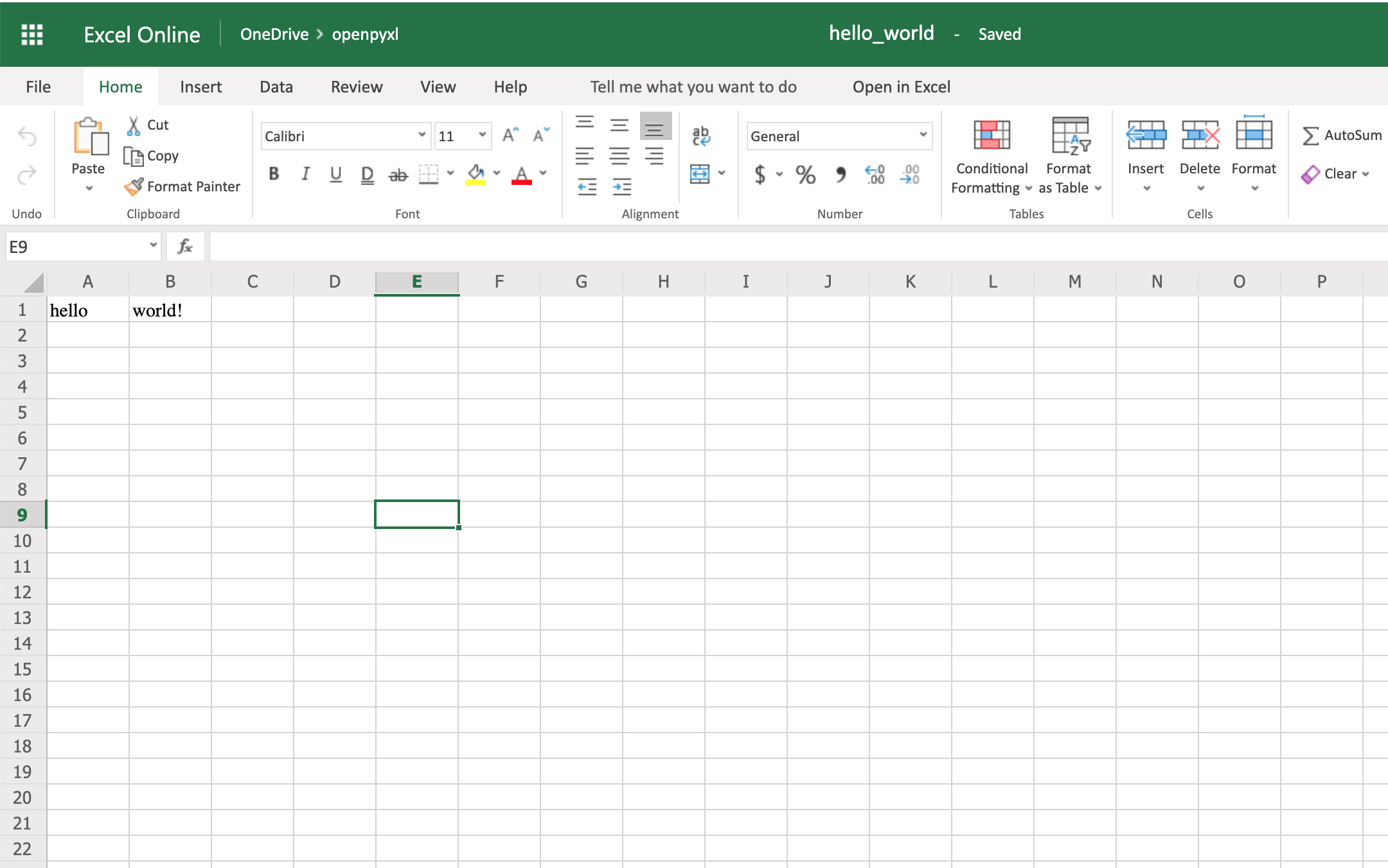 your first spreadsheet created!
Download Dataset: Click here to download the dataset for the openpyxl exercise you'll be following in this tutorial.
your first spreadsheet created!
Download Dataset: Click here to download the dataset for the openpyxl exercise you'll be following in this tutorial.
A Simple Approach to Reading an Excel Spreadsheet
>>>
>>> from openpyxl import load_workbook
>>> workbook = load_workbook(filename="sample.xlsx")
>>> workbook.sheetnames
['Sheet 1']
>>> sheet = workbook.active
>>> sheet
<Worksheet "Sheet 1">
>>> sheet.title
'Sheet 1'
In the code above, you first open the spreadsheet sample.xlsx using load_workbook(), and then you can use workbook.sheetnames to see all the sheets you have available to work with.
After that, workbook.active selects the first available sheet and, in this case, you can see that it selects Sheet 1 automatically.
Using these methods is the default way of opening a spreadsheet, and you'll see it many times during this tutorial.
Now, after opening a spreadsheet, you can easily retrieve data from it like this:
>>>
>>> sheet["A1"]
<Cell 'Sheet 1'.A1>
>>> sheet["A1"].value
'marketplace'
>>> sheet["F10"].value
"G-Shock Men's Grey Sport Watch"
To return the actual value of a cell, you need to do .value.
Otherwise, you'll get the main Cell object.
You can also use the method .cell() to retrieve a cell using index notation.
Remember to add .value to get the actual value and not a Cell object:
>>>
>>> sheet.cell(row=10, column=6)
<Cell 'Sheet 1'.F10>
>>> sheet.cell(row=10, column=6).value
"G-Shock Men's Grey Sport Watch"
You can see that the results returned are the same, no matter which way you decide to go with.
However, in this tutorial, you'll be mostly using the first approach: ["A1"].
Note: Even though in Python you're used to a zero-indexed notation, with spreadsheets you'll always use a one-indexed notation where the first row or column always has index 1. The above shows you the quickest way to open a spreadsheet.
However, you can pass additional parameters to change the way a spreadsheet is loaded.
Additional Reading Options
There are a few arguments you can pass to load_workbook() that change the way a spreadsheet is loaded.
The most important ones are the following two Booleans:
- read_only loads a spreadsheet in read-only mode allowing you to open very large Excel files.
- data_only ignores loading formulas and instead loads only the resulting values.
Importing Data From a Spreadsheet
Now that you've learned the basics about loading a spreadsheet, it's about time you get to the fun part: the iteration and actual usage of the values within the spreadsheet.
This section is where you'll learn all the different ways you can iterate through the data, but also how to convert that data into something usable and, more importantly, how to do it in a Pythonic way.
Iterating Through the Data
There are a few different ways you can iterate through the data depending on your needs.
You can slice the data with a combination of columns and rows:
>>>
>>> sheet["A1:C2"]
((<Cell 'Sheet 1'.A1>, <Cell 'Sheet 1'.B1>, <Cell 'Sheet 1'.C1>),
(<Cell 'Sheet 1'.A2>, <Cell 'Sheet 1'.B2>, <Cell 'Sheet 1'.C2>))
You can get ranges of rows or columns:
>>>
>>> # Get all cells from column A
>>> sheet["A"]
(<Cell 'Sheet 1'.A1>,
<Cell 'Sheet 1'.A2>,
...
<Cell 'Sheet 1'.A99>,
<Cell 'Sheet 1'.A100>)
>>> # Get all cells for a range of columns
>>> sheet["A:B"]
((<Cell 'Sheet 1'.A1>,
<Cell 'Sheet 1'.A2>,
...
<Cell 'Sheet 1'.A99>,
<Cell 'Sheet 1'.A100>),
(<Cell 'Sheet 1'.B1>,
<Cell 'Sheet 1'.B2>,
...
<Cell 'Sheet 1'.B99>,
<Cell 'Sheet 1'.B100>))
>>> # Get all cells from row 5
>>> sheet[5]
(<Cell 'Sheet 1'.A5>,
<Cell 'Sheet 1'.B5>,
...
<Cell 'Sheet 1'.N5>,
<Cell 'Sheet 1'.O5>)
>>> # Get all cells for a range of rows
>>> sheet[5:6]
((<Cell 'Sheet 1'.A5>,
<Cell 'Sheet 1'.B5>,
...
<Cell 'Sheet 1'.N5>,
<Cell 'Sheet 1'.O5>),
(<Cell 'Sheet 1'.A6>,
<Cell 'Sheet 1'.B6>,
...
<Cell 'Sheet 1'.N6>,
<Cell 'Sheet 1'.O6>))
You'll notice that all of the above examples return a tuple.
If you want to refresh your memory on how to handle tuples in Python, check out the article on Lists and Tuples in Python.
There are also multiple ways of using normal Python generators to go through the data.
The main methods you can use to achieve this are:
- .iter_rows()
- .iter_cols()
Both methods can receive the following arguments:
- min_row
- max_row
- min_col
- max_col
These arguments are used to set boundaries for the iteration:
>>>
>>> for row in sheet.iter_rows(min_row=1,
... max_row=2,
... min_col=1,
... max_col=3):
... print(row)
(<Cell 'Sheet 1'.A1>, <Cell 'Sheet 1'.B1>, <Cell 'Sheet 1'.C1>)
(<Cell 'Sheet 1'.A2>, <Cell 'Sheet 1'.B2>, <Cell 'Sheet 1'.C2>)
>>> for column in sheet.iter_cols(min_row=1,
... max_row=2,
... min_col=1,
... max_col=3):
... print(column)
(<Cell 'Sheet 1'.A1>, <Cell 'Sheet 1'.A2>)
(<Cell 'Sheet 1'.B1>, <Cell 'Sheet 1'.B2>)
(<Cell 'Sheet 1'.C1>, <Cell 'Sheet 1'.C2>)
You'll notice that in the first example, when iterating through the rows using .iter_rows(), you get one tuple element per row selected.
While when using .iter_cols() and iterating through columns, you'll get one tuple per column instead.
One additional argument you can pass to both methods is the Boolean values_only.
When it's set to True, the values of the cell are returned, instead of the Cell object:
>>>
>>> for value in sheet.iter_rows(min_row=1,
... max_row=2,
... min_col=1,
... max_col=3,
... values_only=True):
... print(value)
('marketplace', 'customer_id', 'review_id')
('US', 3653882, 'R3O9SGZBVQBV76')
If you want to iterate through the whole dataset, then you can also use the attributes .rows or .columns directly, which are shortcuts to using .iter_rows() and .iter_cols() without any arguments:
>>>
>>> for row in sheet.rows:
... print(row)
(<Cell 'Sheet 1'.A1>, <Cell 'Sheet 1'.B1>, <Cell 'Sheet 1'.C1>
...
<Cell 'Sheet 1'.M100>, <Cell 'Sheet 1'.N100>, <Cell 'Sheet 1'.O100>)
These shortcuts are very useful when you're iterating through the whole dataset.
Manipulate Data Using Python's Default Data Structures
Now that you know the basics of iterating through the data in a workbook, let's look at smart ways of converting that data into Python structures.
As you saw earlier, the result from all iterations comes in the form of tuples.
However, since a tuple is nothing more than a
list that's immutable, you can easily access its data and transform it into other structures.
For example, say you want to extract product information from the sample.xlsx spreadsheet and into a dictionary where each key is a product ID.
A straightforward way to do this is to iterate over all the rows, pick the columns you know are related to product information, and then store that in a dictionary.
Let's code this out!
First of all, have a look at the headers and see what information you care most about:
>>>
>>> for value in sheet.iter_rows(min_row=1,
... max_row=1,
... values_only=True):
... print(value)
('marketplace', 'customer_id', 'review_id', 'product_id', ...)
This code returns a list of all the column names you have in the spreadsheet.
To start, grab the columns with names:
- product_id
- product_parent
- product_title
- product_category
Lucky for you, the columns you need are all next to each other so you can use the min_column and max_column to easily get the data you want:
>>>
>>> for value in sheet.iter_rows(min_row=2,
... min_col=4,
... max_col=7,
... values_only=True):
... print(value)
('B00FALQ1ZC', 937001370, 'Invicta Women\'s 15150 "Angel" 18k Yellow...)
('B00D3RGO20', 484010722, "Kenneth Cole New York Women's KC4944...)
...
Nice! Now that you know how to get all the important product information you need, let's put that data into a dictionary:
import json
from openpyxl import load_workbook
workbook = load_workbook(filename="sample.xlsx")
sheet = workbook.active
products = {}
# Using the values_only because you want to return the cells' values
for row in sheet.iter_rows(min_row=2,
min_col=4,
max_col=7,
values_only=True):
product_id = row[0]
product = {
"parent": row[1],
"title": row[2],
"category": row[3]
}
products[product_id] = product
# Using json here to be able to format the output for displaying later
print(json.dumps(products))
The code above returns a JSON similar to this:
{
"B00FALQ1ZC": {
"parent": 937001370,
"title": "Invicta Women's 15150 ...",
"category": "Watches"
},
"B00D3RGO20": {
"parent": 484010722,
"title": "Kenneth Cole New York ...",
"category": "Watches"
}
}
Here you can see that the output is trimmed to 2 products only, but if you run the script as it is, then you should get 98 products.
Convert Data Into Python Classes
To finalize the reading section of this tutorial, let's dive into Python classes and see how you could improve on the example above and better structure the data.
For this, you'll be using the new Python Data Classes that are available from Python 3.7.
If you're using an older version of Python, then you can use the default Classes instead.
So, first things first, let's look at the data you have and decide what you want to store and how you want to store it.
As you saw right at the start, this data comes from Amazon, and it's a list of product reviews.
You can check the list of all the columns and their meaning on Amazon.
There are two significant elements you can extract from the data available:
- Products
- Reviews
A Product has:
- ID
- Title
- Parent
- Category
The Review has a few more fields:
- ID
- Customer ID
- Stars
- Headline
- Body
- Date
You can ignore a few of the review fields to make things a bit simpler.
So, a straightforward implementation of these two classes could be written in a separate file classes.py:
import datetime
from dataclasses import dataclass
@dataclass
class Product:
id: str
parent: str
title: str
category: str
@dataclass
class Review:
id: str
customer_id: str
stars: int
headline: str
body: str
date: datetime.datetime
After defining your data classes, you need to convert the data from the spreadsheet into these new structures.
Before doing the conversion, it's worth looking at our header again and creating a mapping between columns and the fields you need:
>>>
>>> for value in sheet.iter_rows(min_row=1,
... max_row=1,
... values_only=True):
... print(value)
('marketplace', 'customer_id', 'review_id', 'product_id', ...)
>>> # Or an alternative
>>> for cell in sheet[1]:
... print(cell.value)
marketplace
customer_id
review_id
product_id
product_parent
...
Let's create a file mapping.py where you have a list of all the field names and their column location (zero-indexed) on the spreadsheet:
# Product fields
PRODUCT_ID = 3
PRODUCT_PARENT = 4
PRODUCT_TITLE = 5
PRODUCT_CATEGORY = 6
# Review fields
REVIEW_ID = 2
REVIEW_CUSTOMER = 1
REVIEW_STARS = 7
REVIEW_HEADLINE = 12
REVIEW_BODY = 13
REVIEW_DATE = 14
You don't necessarily have to do the mapping above.
It's more for readability when parsing the row data, so you don't end up with a lot of magic numbers lying around.
Finally, let's look at the code needed to parse the spreadsheet data into a list of product and review objects:
from datetime import datetime
from openpyxl import load_workbook
from classes import Product, Review
from mapping import PRODUCT_ID, PRODUCT_PARENT, PRODUCT_TITLE, \
PRODUCT_CATEGORY, REVIEW_DATE, REVIEW_ID, REVIEW_CUSTOMER, \
REVIEW_STARS, REVIEW_HEADLINE, REVIEW_BODY
# Using the read_only method since you're not gonna be editing the spreadsheet
workbook = load_workbook(filename="sample.xlsx", read_only=True)
sheet = workbook.active
products = []
reviews = []
# Using the values_only because you just want to return the cell value
for row in sheet.iter_rows(min_row=2, values_only=True):
product = Product(id=row[PRODUCT_ID],
parent=row[PRODUCT_PARENT],
title=row[PRODUCT_TITLE],
category=row[PRODUCT_CATEGORY])
products.append(product)
# You need to parse the date from the spreadsheet into a datetime format
spread_date = row[REVIEW_DATE]
parsed_date = datetime.strptime(spread_date, "%Y-%m-%d")
review = Review(id=row[REVIEW_ID],
customer_id=row[REVIEW_CUSTOMER],
stars=row[REVIEW_STARS],
headline=row[REVIEW_HEADLINE],
body=row[REVIEW_BODY],
date=parsed_date)
reviews.append(review)
print(products[0])
print(reviews[0])
After you run the code above, you should get some output like this:
Product(id='B00FALQ1ZC', parent=937001370, ...)
Review(id='R3O9SGZBVQBV76', customer_id=3653882, ...)
That's it! Now you should have the data in a very simple and digestible class format, and you can start thinking of storing this in a Database or any other type of data storage you like.
Using this kind of OOP strategy to parse spreadsheets makes handling the data much simpler later on.
Appending New Data
Before you start creating very complex spreadsheets, have a quick look at an example of how to append data to an existing spreadsheet.
Go back to the first example spreadsheet you created (
hello_world.xlsx) and try opening it and appending some data to it, like this:
from openpyxl import load_workbook
# Start by opening the spreadsheet and selecting the main sheet
workbook = load_workbook(filename="hello_world.xlsx")
sheet = workbook.active
# Write what you want into a specific cell
sheet["C1"] = "writing ;)"
# Save the spreadsheet
workbook.save(filename="hello_world_append.xlsx")
Et voilà, if you open the new hello_world_append.xlsx spreadsheet, you'll see the following change:
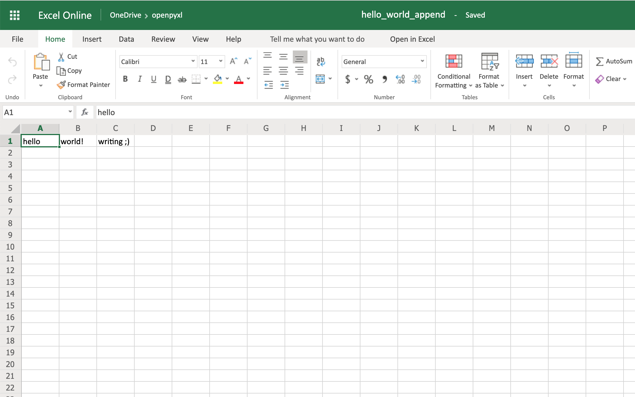 Notice the additional writing ;) on cell C1.
Writing Excel Spreadsheets With openpyxl
There are a lot of different things you can write to a spreadsheet, from simple text or number values to complex formulas, charts, or even images.
Let's start creating some spreadsheets!
Creating a Simple Spreadsheet
Previously, you saw a very quick example of how to write “Hello world!” into a spreadsheet, so you can start with that:
1from openpyxl import Workbook
2
3filename = "hello_world.xlsx"
4
5workbook = Workbook()
6sheet = workbook.active
7
8sheet["A1"] = "hello"
9sheet["B1"] = "world!"
10
11workbook.save(filename=filename)
The highlighted lines in the code above are the most important ones for writing.
In the code, you can see that:
- Line 5 shows you how to create a new empty workbook.
- Lines 8 and 9 show you how to add data to specific cells.
- Line 11 shows you how to save the spreadsheet when you're done.
Even though these lines above can be straightforward, it's still good to know them well for when things get a bit more complicated.
Note: You'll be using the hello_world.xlsx spreadsheet for some of the upcoming examples, so keep it handy.
One thing you can do to help with coming code examples is add the following method to your Python file or console:
>>>
>>> def print_rows():
... for row in sheet.iter_rows(values_only=True):
... print(row)
It makes it easier to print all of your spreadsheet values by just calling print_rows().
Basic Spreadsheet Operations
Before you get into the more advanced topics, it's good for you to know how to manage the most simple elements of a spreadsheet.
Adding and Updating Cell Values
You already learned how to add values to a spreadsheet like this:
>>>
>>> sheet["A1"] = "value"
There's another way you can do this, by first selecting a cell and then changing its value:
>>>
>>> cell = sheet["A1"]
>>> cell
<Cell 'Sheet'.A1>
>>> cell.value
'hello'
>>> cell.value = "hey"
>>> cell.value
'hey'
The new value is only stored into the spreadsheet once you call workbook.save().
The openpyxl creates a cell when adding a value, if that cell didn't exist before:
>>>
>>> # Before, our spreadsheet has only 1 row
>>> print_rows()
('hello', 'world!')
>>> # Try adding a value to row 10
>>> sheet["B10"] = "test"
>>> print_rows()
('hello', 'world!')
(None, None)
(None, None)
(None, None)
(None, None)
(None, None)
(None, None)
(None, None)
(None, None)
(None, 'test')
As you can see, when trying to add a value to cell B10, you end up with a tuple with 10 rows, just so you can have that test value.
Managing Rows and Columns
One of the most common things you have to do when manipulating spreadsheets is adding or removing rows and columns.
The openpyxl package allows you to do that in a very straightforward way by using the methods:
- .insert_rows()
- .delete_rows()
- .insert_cols()
- .delete_cols()
Every single one of those methods can receive two arguments:
- idx
- amount
Using our basic hello_world.xlsx example again, let's see how these methods work:
>>>
>>> print_rows()
('hello', 'world!')
>>> # Insert a column before the existing column 1 ("A")
>>> sheet.insert_cols(idx=1)
>>> print_rows()
(None, 'hello', 'world!')
>>> # Insert 5 columns between column 2 ("B") and 3 ("C")
>>> sheet.insert_cols(idx=3, amount=5)
>>> print_rows()
(None, 'hello', None, None, None, None, None, 'world!')
>>> # Delete the created columns
>>> sheet.delete_cols(idx=3, amount=5)
>>> sheet.delete_cols(idx=1)
>>> print_rows()
('hello', 'world!')
>>> # Insert a new row in the beginning
>>> sheet.insert_rows(idx=1)
>>> print_rows()
(None, None)
('hello', 'world!')
>>> # Insert 3 new rows in the beginning
>>> sheet.insert_rows(idx=1, amount=3)
>>> print_rows()
(None, None)
(None, None)
(None, None)
(None, None)
('hello', 'world!')
>>> # Delete the first 4 rows
>>> sheet.delete_rows(idx=1, amount=4)
>>> print_rows()
('hello', 'world!')
The only thing you need to remember is that when inserting new data (rows or columns), the insertion happens before the idx parameter.
So, if you do insert_rows(1), it inserts a new row before the existing first row.
It's the same for columns: when you call insert_cols(2), it inserts a new column right before the already existing second column (
B).
However, when deleting rows or columns, .delete_... deletes data starting from the index passed as an argument.
For example, when doing delete_rows(2) it deletes row 2, and when doing delete_cols(3) it deletes the third column (
C).
Managing Sheets
Sheet management is also one of those things you might need to know, even though it might be something that you don't use that often.
If you look back at the code examples from this tutorial, you'll notice the following recurring piece of code:
sheet = workbook.active
This is the way to select the default sheet from a spreadsheet.
However, if you're opening a spreadsheet with multiple sheets, then you can always select a specific one like this:
>>>
>>> # Let's say you have two sheets: "Products" and "Company Sales"
>>> workbook.sheetnames
['Products', 'Company Sales']
>>> # You can select a sheet using its title
>>> products_sheet = workbook["Products"]
>>> sales_sheet = workbook["Company Sales"]
You can also change a sheet title very easily:
>>>
>>> workbook.sheetnames
['Products', 'Company Sales']
>>> products_sheet = workbook["Products"]
>>> products_sheet.title = "New Products"
>>> workbook.sheetnames
['New Products', 'Company Sales']
If you want to create or delete sheets, then you can also do that with .create_sheet() and .remove():
>>>
>>> workbook.sheetnames
['Products', 'Company Sales']
>>> operations_sheet = workbook.create_sheet("Operations")
>>> workbook.sheetnames
['Products', 'Company Sales', 'Operations']
>>> # You can also define the position to create the sheet at
>>> hr_sheet = workbook.create_sheet("HR", 0)
>>> workbook.sheetnames
['HR', 'Products', 'Company Sales', 'Operations']
>>> # To remove them, just pass the sheet as an argument to the .remove()
>>> workbook.remove(operations_sheet)
>>> workbook.sheetnames
['HR', 'Products', 'Company Sales']
>>> workbook.remove(hr_sheet)
>>> workbook.sheetnames
['Products', 'Company Sales']
One other thing you can do is make duplicates of a sheet using copy_worksheet():
>>>
>>> workbook.sheetnames
['Products', 'Company Sales']
>>> products_sheet = workbook["Products"]
>>> workbook.copy_worksheet(products_sheet)
<Worksheet "Products Copy">
>>> workbook.sheetnames
['Products', 'Company Sales', 'Products Copy']
If you open your spreadsheet after saving the above code, you'll notice that the sheet Products Copy is a duplicate of the sheet Products.
Freezing Rows and Columns
Something that you might want to do when working with big spreadsheets is to freeze a few rows or columns, so they remain visible when you scroll right or down.
Freezing data allows you to keep an eye on important rows or columns, regardless of where you scroll in the spreadsheet.
Again, openpyxl also has a way to accomplish this by using the worksheet freeze_panes attribute.
For this example, go back to our sample.xlsx spreadsheet and try doing the following:
>>>
>>> workbook = load_workbook(filename="sample.xlsx")
>>> sheet = workbook.active
>>> sheet.freeze_panes = "C2"
>>> workbook.save("sample_frozen.xlsx")
If you open the sample_frozen.xlsx spreadsheet in your favorite spreadsheet editor, you'll notice that row 1 and columns A and B are frozen and are always visible no matter where you navigate within the spreadsheet.
This feature is handy, for example, to keep headers within sight, so you always know what each column represents.
Here's how it looks in the editor:
 Notice how you're at the end of the spreadsheet, and yet, you can see both row 1 and columns A and B.
Adding Filters
You can use openpyxl to add filters and sorts to your spreadsheet.
However, when you open the spreadsheet, the data won't be rearranged according to these sorts and filters.
At first, this might seem like a pretty useless feature, but when you're programmatically creating a spreadsheet that is going to be sent and used by somebody else, it's still nice to at least create the filters and allow people to use it afterward.
The code below is an example of how you would add some filters to our existing sample.xlsx spreadsheet:
>>>
>>> # Check the used spreadsheet space using the attribute "dimensions"
>>> sheet.dimensions
'A1:O100'
>>> sheet.auto_filter.ref = "A1:O100"
>>> workbook.save(filename="sample_with_filters.xlsx")
You should now see the filters created when opening the spreadsheet in your editor:
 You don't have to use sheet.dimensions if you know precisely which part of the spreadsheet you want to apply filters to.
Adding Formulas
Formulas (or formulae) are one of the most powerful features of spreadsheets.
They gives you the power to apply specific mathematical equations to a range of cells.
Using formulas with openpyxl is as simple as editing the value of a cell.
You can see the list of formulas supported by openpyxl:
>>>
>>> from openpyxl.utils import FORMULAE
>>> FORMULAE
frozenset({'ABS',
'ACCRINT',
'ACCRINTM',
'ACOS',
'ACOSH',
'AMORDEGRC',
'AMORLINC',
'AND',
...
'YEARFRAC',
'YIELD',
'YIELDDISC',
'YIELDMAT',
'ZTEST'})
Let's add some formulas to our sample.xlsx spreadsheet.
Starting with something easy, let's check the average star rating for the 99 reviews within the spreadsheet:
>>>
>>> # Star rating is column "H"
>>> sheet["P2"] = "=AVERAGE(H2:H100)"
>>> workbook.save(filename="sample_formulas.xlsx")
If you open the spreadsheet now and go to cell P2, you should see that its value is: 4.18181818181818.
Have a look in the editor:
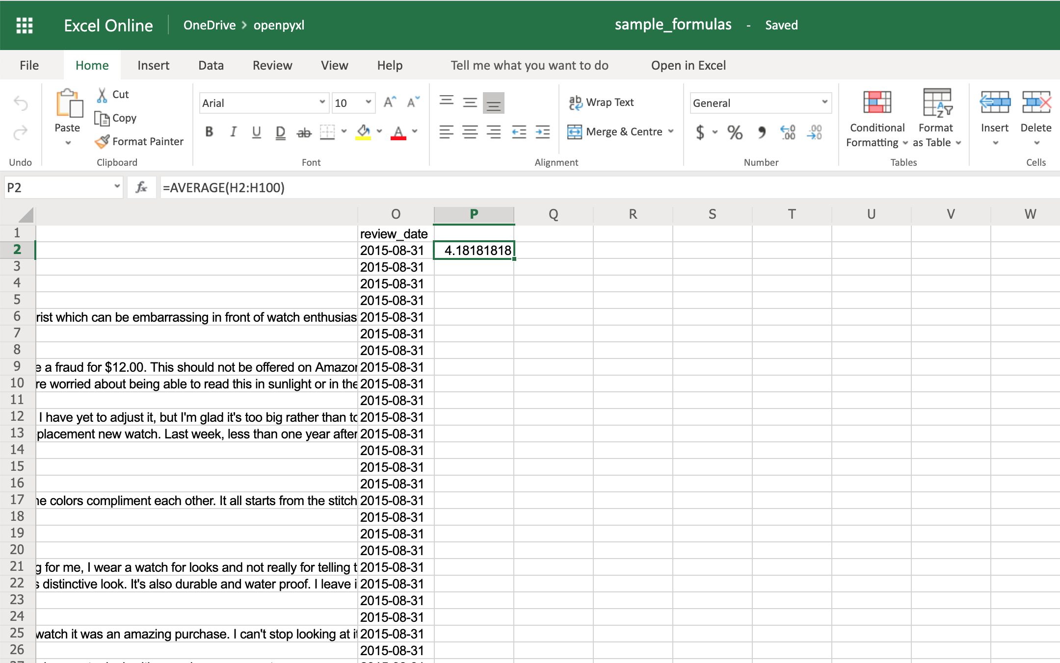 You can use the same methodology to add any formulas to your spreadsheet.
For example, let's count the number of reviews that had helpful votes:
>>>
>>> # The helpful votes are counted on column "I"
>>> sheet["P3"] = '=COUNTIF(I2:I100, ">0")'
>>> workbook.save(filename="sample_formulas.xlsx")
You should get the number 21 on your P3 spreadsheet cell like so:
You can use the same methodology to add any formulas to your spreadsheet.
For example, let's count the number of reviews that had helpful votes:
>>>
>>> # The helpful votes are counted on column "I"
>>> sheet["P3"] = '=COUNTIF(I2:I100, ">0")'
>>> workbook.save(filename="sample_formulas.xlsx")
You should get the number 21 on your P3 spreadsheet cell like so:
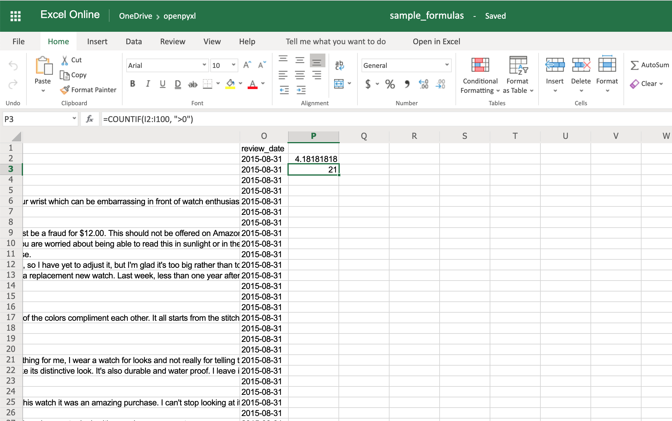 You'll have to make sure that the strings within a formula are always in double quotes, so you either have to use single quotes around the formula like in the example above or you'll have to escape the double quotes inside the formula: "=COUNTIF(I2:I100, \">0\")".
There are a ton of other formulas you can add to your spreadsheet using the same procedure you tried above.
Give it a go yourself!
You'll have to make sure that the strings within a formula are always in double quotes, so you either have to use single quotes around the formula like in the example above or you'll have to escape the double quotes inside the formula: "=COUNTIF(I2:I100, \">0\")".
There are a ton of other formulas you can add to your spreadsheet using the same procedure you tried above.
Give it a go yourself!
Adding Styles
Even though styling a spreadsheet might not be something you would do every day, it's still good to know how to do it.
Using openpyxl, you can apply multiple styling options to your spreadsheet, including fonts, borders, colors, and so on.
Have a look at the openpyxl documentation to learn more.
You can also choose to either apply a style directly to a cell or create a template and reuse it to apply styles to multiple cells.
Let's start by having a look at simple cell styling, using our sample.xlsx again as the base spreadsheet:
>>>
>>> # Import necessary style classes
>>> from openpyxl.styles import Font, Color, Alignment, Border, Side
>>> # Create a few styles
>>> bold_font = Font(bold=True)
>>> big_red_text = Font(color="00FF0000", size=20)
>>> center_aligned_text = Alignment(horizontal="center")
>>> double_border_side = Side(border_style="double")
>>> square_border = Border(top=double_border_side,
... right=double_border_side,
... bottom=double_border_side,
... left=double_border_side)
>>> # Style some cells!
>>> sheet["A2"].font = bold_font
>>> sheet["A3"].font = big_red_text
>>> sheet["A4"].alignment = center_aligned_text
>>> sheet["A5"].border = square_border
>>> workbook.save(filename="sample_styles.xlsx")
If you open your spreadsheet now, you should see quite a few different styles on the first 5 cells of column A:
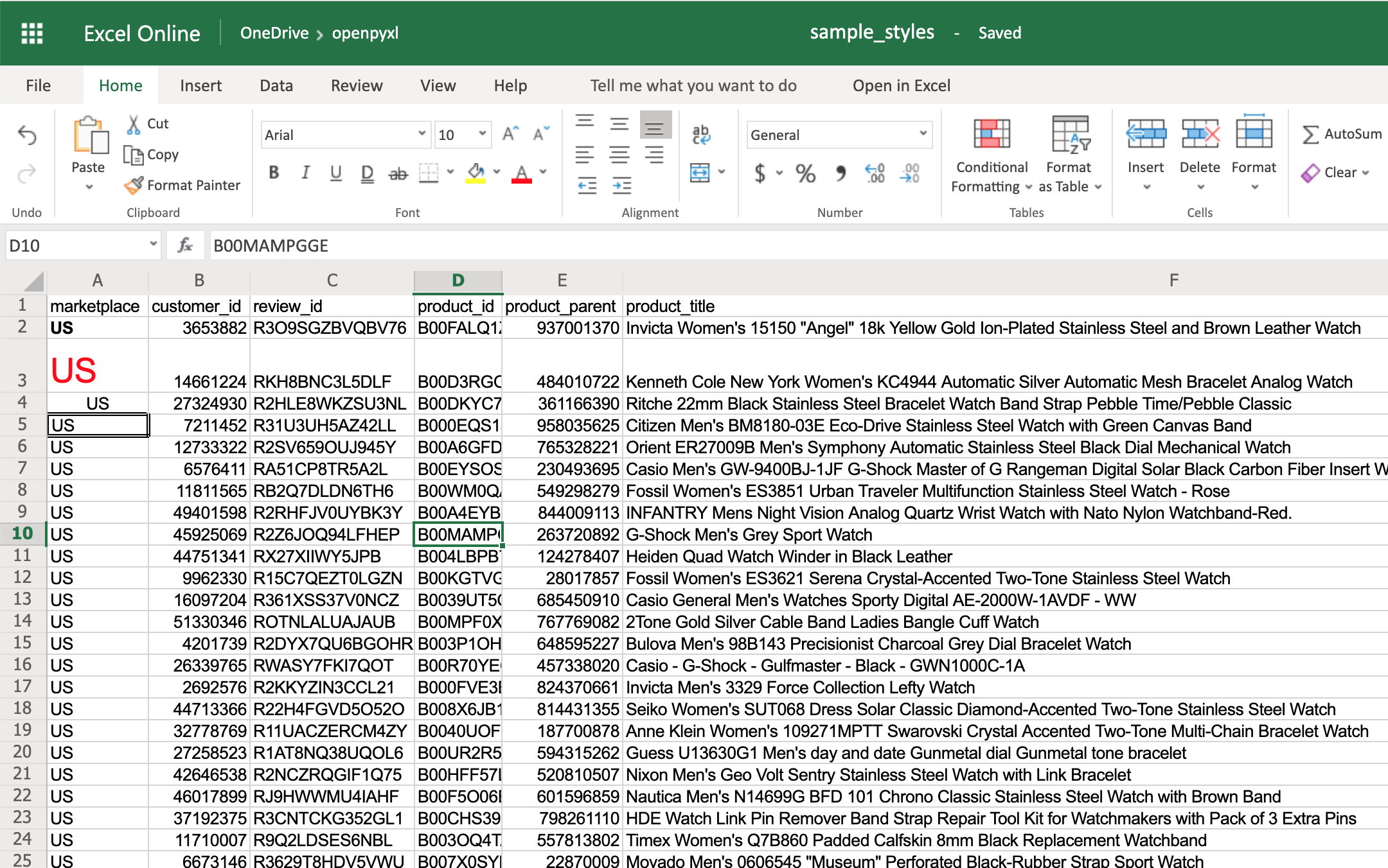 There you go.
You got:
There you go.
You got:
- A2 with the text in bold
- A3 with the text in red and bigger font size
- A4 with the text centered
- A5 with a square border around the text
Note: For the colors, you can also use HEX codes instead by doing Font(color="C70E0F").
You can also combine styles by simply adding them to the cell at the same time:
>>>
>>> # Reusing the same styles from the example above
>>> sheet["A6"].alignment = center_aligned_text
>>> sheet["A6"].font = big_red_text
>>> sheet["A6"].border = square_border
>>> workbook.save(filename="sample_styles.xlsx")
Have a look at cell A6 here:
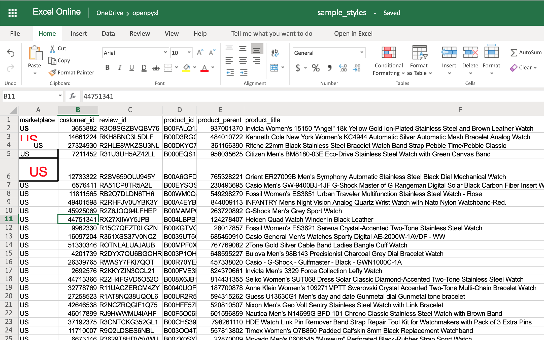 When you want to apply multiple styles to one or several cells, you can use a NamedStyle class instead, which is like a style template that you can use over and over again.
Have a look at the example below:
>>>
>>> from openpyxl.styles import NamedStyle
>>> # Let's create a style template for the header row
>>> header = NamedStyle(name="header")
>>> header.font = Font(bold=True)
>>> header.border = Border(bottom=Side(border_style="thin"))
>>> header.alignment = Alignment(horizontal="center", vertical="center")
>>> # Now let's apply this to all first row (header) cells
>>> header_row = sheet[1]
>>> for cell in header_row:
... cell.style = header
>>> workbook.save(filename="sample_styles.xlsx")
If you open the spreadsheet now, you should see that its first row is bold, the text is aligned to the center, and there's a small bottom border! Have a look below:
When you want to apply multiple styles to one or several cells, you can use a NamedStyle class instead, which is like a style template that you can use over and over again.
Have a look at the example below:
>>>
>>> from openpyxl.styles import NamedStyle
>>> # Let's create a style template for the header row
>>> header = NamedStyle(name="header")
>>> header.font = Font(bold=True)
>>> header.border = Border(bottom=Side(border_style="thin"))
>>> header.alignment = Alignment(horizontal="center", vertical="center")
>>> # Now let's apply this to all first row (header) cells
>>> header_row = sheet[1]
>>> for cell in header_row:
... cell.style = header
>>> workbook.save(filename="sample_styles.xlsx")
If you open the spreadsheet now, you should see that its first row is bold, the text is aligned to the center, and there's a small bottom border! Have a look below:
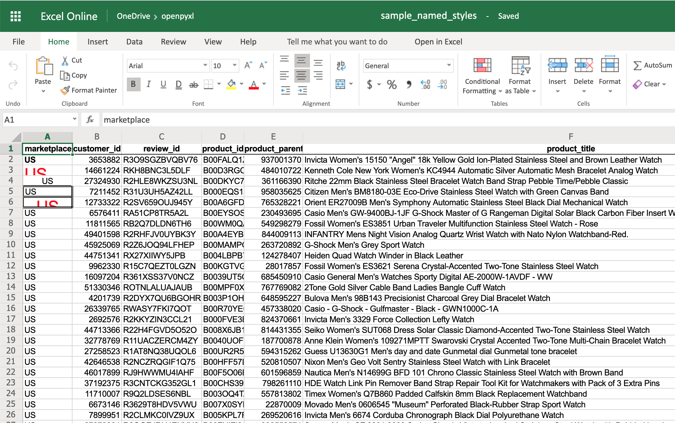 As you saw above, there are many options when it comes to styling, and it depends on the use case, so feel free to check openpyxl documentation and see what other things you can do.
Conditional Formatting
This feature is one of my personal favorites when it comes to adding styles to a spreadsheet.
It's a much more powerful approach to styling because it dynamically applies styles according to how the data in the spreadsheet changes.
In a nutshell, conditional formatting allows you to specify a list of styles to apply to a cell (or cell range) according to specific conditions.
For example, a widespread use case is to have a balance sheet where all the negative totals are in red, and the positive ones are in green.
This formatting makes it much more efficient to spot good vs bad periods.
Without further ado, let's pick our favorite spreadsheet—
sample.xlsx—and add some conditional formatting.
You can start by adding a simple one that adds a red background to all reviews with less than 3 stars:
>>>
>>> from openpyxl.styles import PatternFill
>>> from openpyxl.styles.differential import DifferentialStyle
>>> from openpyxl.formatting.rule import Rule
>>> red_background = PatternFill(fgColor="00FF0000")
>>> diff_style = DifferentialStyle(fill=red_background)
>>> rule = Rule(type="expression", dxf=diff_style)
>>> rule.formula = ["$H1<3"]
>>> sheet.conditional_formatting.add("A1:O100", rule)
>>> workbook.save("sample_conditional_formatting.xlsx")
Now you'll see all the reviews with a star rating below 3 marked with a red background:
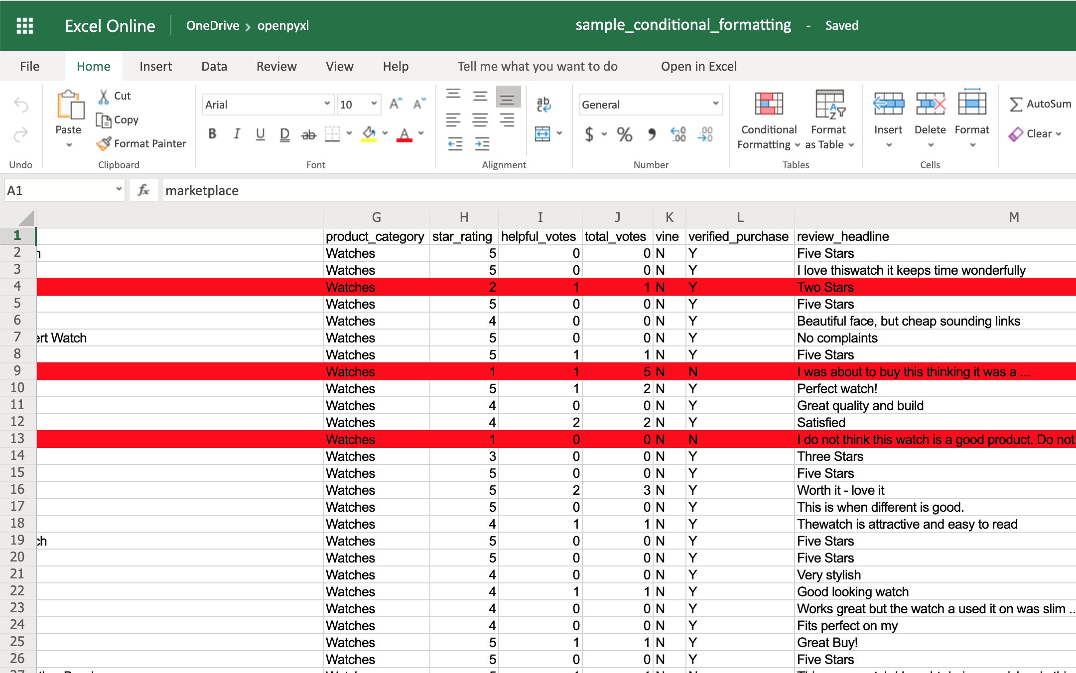 Code-wise, the only things that are new here are the objects DifferentialStyle and Rule:
-
DifferentialStyle is quite similar to NamedStyle, which you already saw above, and it's used to aggregate multiple styles such as fonts, borders, alignment, and so forth.
-
Rule is responsible for selecting the cells and applying the styles if the cells match the rule's logic.
Using a Rule object, you can create numerous conditional formatting scenarios.
However, for simplicity sake, the openpyxl package offers 3 built-in formats that make it easier to create a few common conditional formatting patterns.
These built-ins are:
- ColorScale
- IconSet
- DataBar
The ColorScale gives you the ability to create color gradients:
>>>
>>> from openpyxl.formatting.rule import ColorScaleRule
>>> color_scale_rule = ColorScaleRule(start_type="min",
... start_color="00FF0000", # Red
... end_type="max",
... end_color="0000FF00") # Green
>>> # Again, let's add this gradient to the star ratings, column "H"
>>> sheet.conditional_formatting.add("H2:H100", color_scale_rule)
>>> workbook.save(filename="sample_conditional_formatting_color_scale.xlsx")
Now you should see a color gradient on column H, from red to green, according to the star rating:
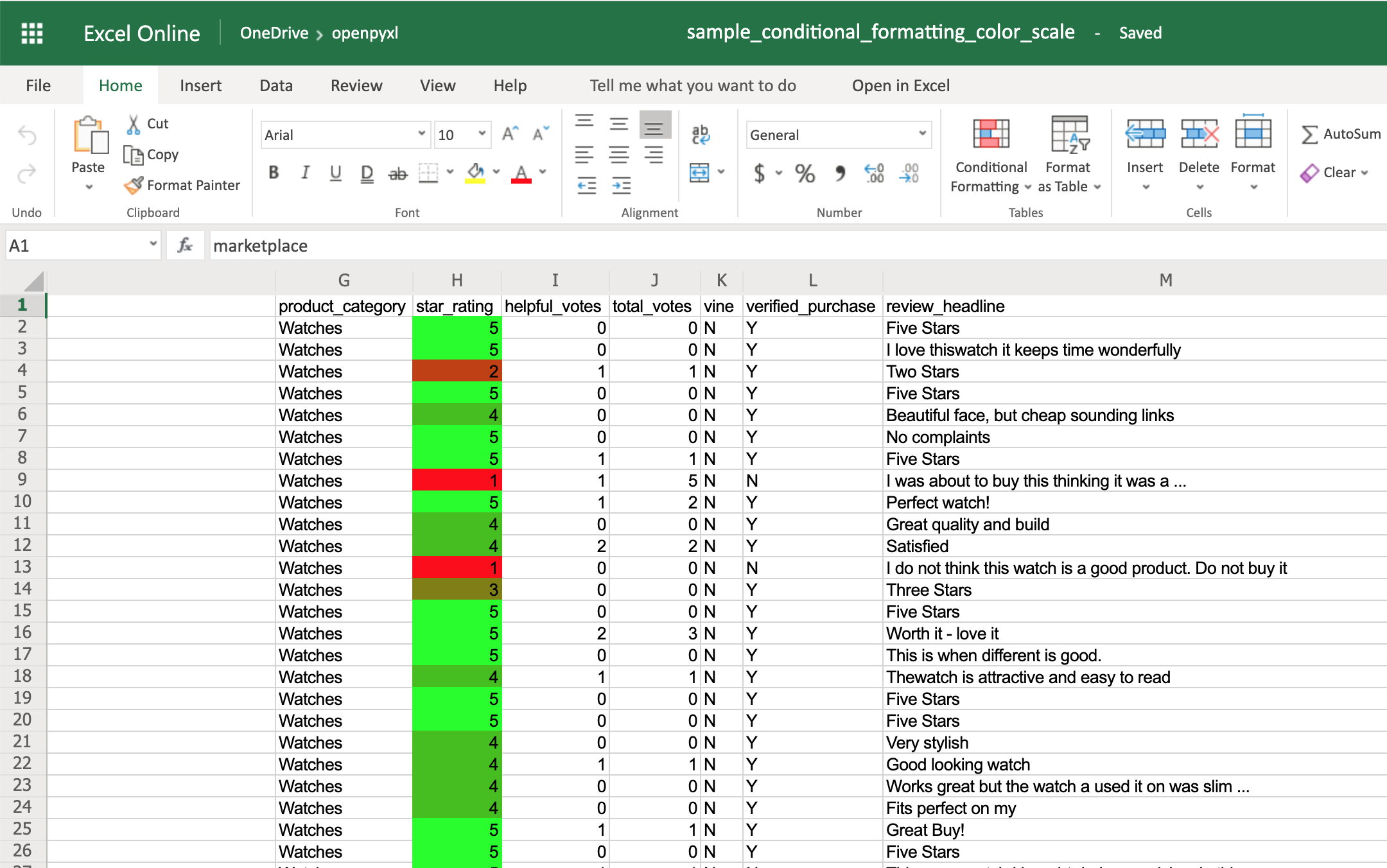 You can also add a third color and make two gradients instead:
>>>
>>> from openpyxl.formatting.rule import ColorScaleRule
>>> color_scale_rule = ColorScaleRule(start_type="num",
... start_value=1,
... start_color="00FF0000", # Red
... mid_type="num",
... mid_value=3,
... mid_color="00FFFF00", # Yellow
... end_type="num",
... end_value=5,
... end_color="0000FF00") # Green
>>> # Again, let's add this gradient to the star ratings, column "H"
>>> sheet.conditional_formatting.add("H2:H100", color_scale_rule)
>>> workbook.save(filename="sample_conditional_formatting_color_scale_3.xlsx")
This time, you'll notice that star ratings between 1 and 3 have a gradient from red to yellow, and star ratings between 3 and 5 have a gradient from yellow to green:
You can also add a third color and make two gradients instead:
>>>
>>> from openpyxl.formatting.rule import ColorScaleRule
>>> color_scale_rule = ColorScaleRule(start_type="num",
... start_value=1,
... start_color="00FF0000", # Red
... mid_type="num",
... mid_value=3,
... mid_color="00FFFF00", # Yellow
... end_type="num",
... end_value=5,
... end_color="0000FF00") # Green
>>> # Again, let's add this gradient to the star ratings, column "H"
>>> sheet.conditional_formatting.add("H2:H100", color_scale_rule)
>>> workbook.save(filename="sample_conditional_formatting_color_scale_3.xlsx")
This time, you'll notice that star ratings between 1 and 3 have a gradient from red to yellow, and star ratings between 3 and 5 have a gradient from yellow to green:
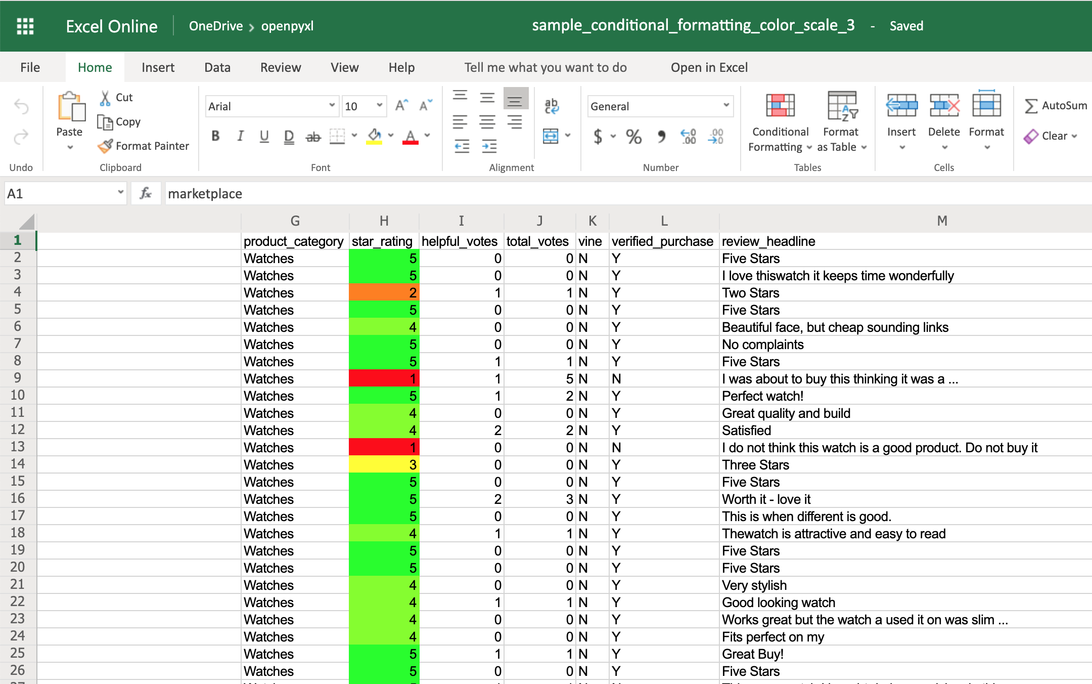 The IconSet allows you to add an icon to the cell according to its value:
>>>
>>> from openpyxl.formatting.rule import IconSetRule
>>> icon_set_rule = IconSetRule("5Arrows", "num", [1, 2, 3, 4, 5])
>>> sheet.conditional_formatting.add("H2:H100", icon_set_rule)
>>> workbook.save("sample_conditional_formatting_icon_set.xlsx")
You'll see a colored arrow next to the star rating.
This arrow is red and points down when the value of the cell is 1 and, as the rating gets better, the arrow starts pointing up and becomes green:
The IconSet allows you to add an icon to the cell according to its value:
>>>
>>> from openpyxl.formatting.rule import IconSetRule
>>> icon_set_rule = IconSetRule("5Arrows", "num", [1, 2, 3, 4, 5])
>>> sheet.conditional_formatting.add("H2:H100", icon_set_rule)
>>> workbook.save("sample_conditional_formatting_icon_set.xlsx")
You'll see a colored arrow next to the star rating.
This arrow is red and points down when the value of the cell is 1 and, as the rating gets better, the arrow starts pointing up and becomes green:
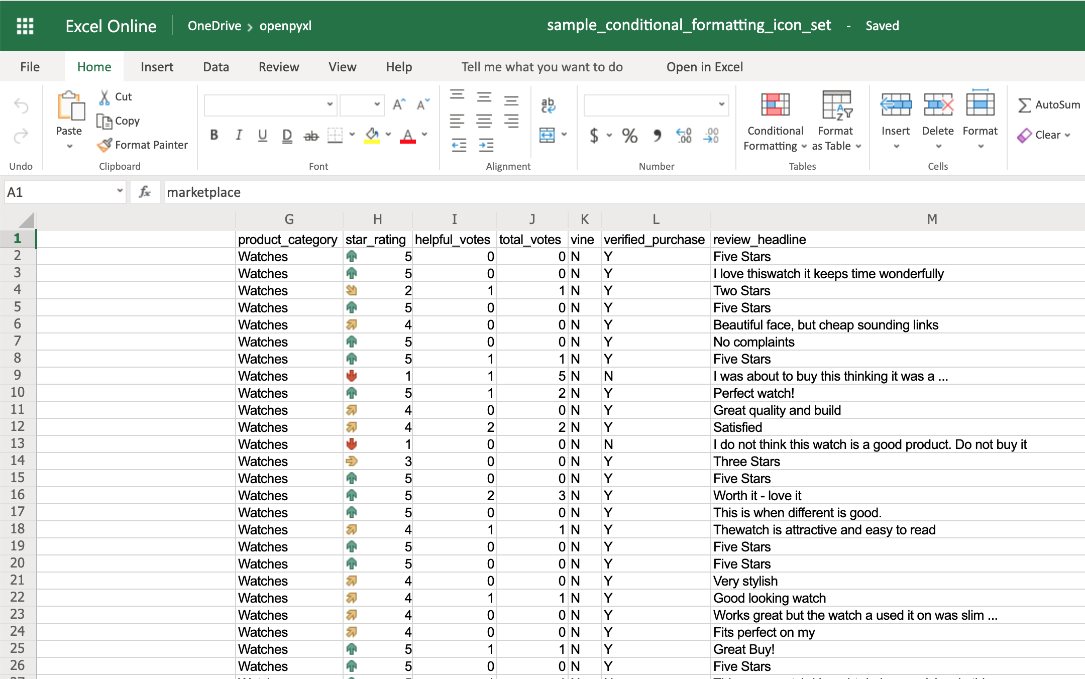 The openpyxl package has a full list of other icons you can use, besides the arrow.
Finally, the DataBar allows you to create progress bars:
>>>
>>> from openpyxl.formatting.rule import DataBarRule
>>> data_bar_rule = DataBarRule(start_type="num",
... start_value=1,
... end_type="num",
... end_value="5",
... color="0000FF00") # Green
>>> sheet.conditional_formatting.add("H2:H100", data_bar_rule)
>>> workbook.save("sample_conditional_formatting_data_bar.xlsx")
You'll now see a green progress bar that gets fuller the closer the star rating is to the number 5:
The openpyxl package has a full list of other icons you can use, besides the arrow.
Finally, the DataBar allows you to create progress bars:
>>>
>>> from openpyxl.formatting.rule import DataBarRule
>>> data_bar_rule = DataBarRule(start_type="num",
... start_value=1,
... end_type="num",
... end_value="5",
... color="0000FF00") # Green
>>> sheet.conditional_formatting.add("H2:H100", data_bar_rule)
>>> workbook.save("sample_conditional_formatting_data_bar.xlsx")
You'll now see a green progress bar that gets fuller the closer the star rating is to the number 5:
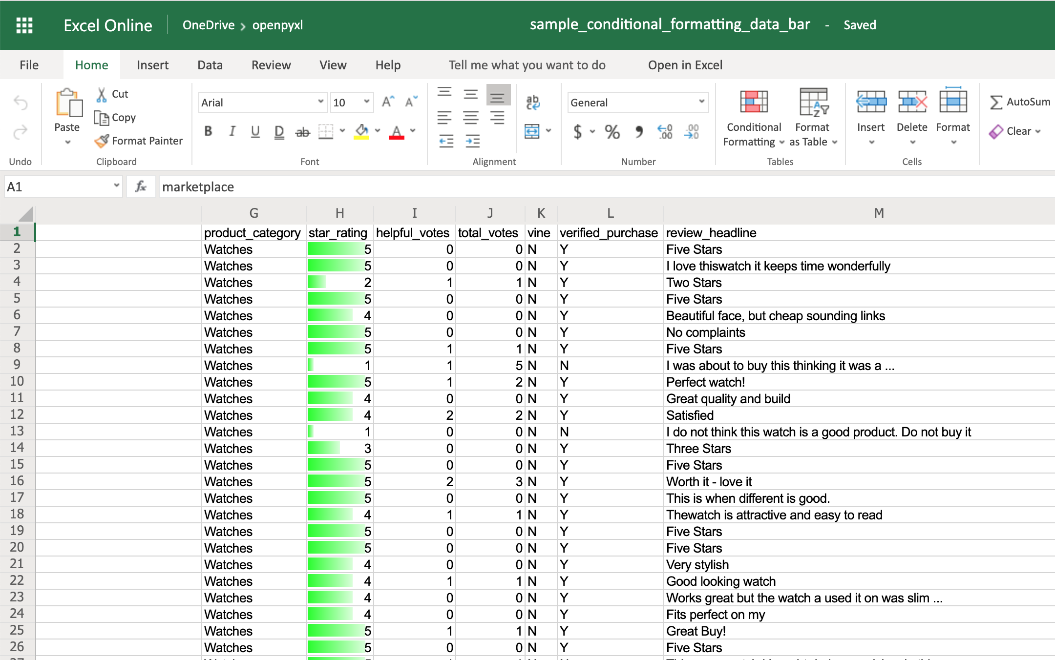 As you can see, there are a lot of cool things you can do with conditional formatting.
Here, you saw only a few examples of what you can achieve with it, but check the openpyxl documentation to see a bunch of other options.
As you can see, there are a lot of cool things you can do with conditional formatting.
Here, you saw only a few examples of what you can achieve with it, but check the openpyxl documentation to see a bunch of other options.
Adding Images
Even though images are not something that you'll often see in a spreadsheet, it's quite cool to be able to add them.
Maybe you can use it for branding purposes or to make spreadsheets more personal.
To be able to load images to a spreadsheet using openpyxl, you'll have to install Pillow:
$ pip install Pillow
Apart from that, you'll also need an image.
For this example, you can grab the Real Python logo below and convert it from .webp to .png using an online converter such as cloudconvert.com, save the final file as logo.png, and copy it to the root folder where you're running your examples:
 Afterward, this is the code you need to import that image into the hello_word.xlsx spreadsheet:
from openpyxl import load_workbook
from openpyxl.drawing.image import Image
# Let's use the hello_world spreadsheet since it has less data
workbook = load_workbook(filename="hello_world.xlsx")
sheet = workbook.active
logo = Image("logo.png")
# A bit of resizing to not fill the whole spreadsheet with the logo
logo.height = 150
logo.width = 150
sheet.add_image(logo, "A3")
workbook.save(filename="hello_world_logo.xlsx")
You have an image on your spreadsheet! Here it is:
Afterward, this is the code you need to import that image into the hello_word.xlsx spreadsheet:
from openpyxl import load_workbook
from openpyxl.drawing.image import Image
# Let's use the hello_world spreadsheet since it has less data
workbook = load_workbook(filename="hello_world.xlsx")
sheet = workbook.active
logo = Image("logo.png")
# A bit of resizing to not fill the whole spreadsheet with the logo
logo.height = 150
logo.width = 150
sheet.add_image(logo, "A3")
workbook.save(filename="hello_world_logo.xlsx")
You have an image on your spreadsheet! Here it is:
 The image's left top corner is on the cell you chose, in this case, A3.
Adding Pretty Charts
Another powerful thing you can do with spreadsheets is create an incredible variety of charts.
Charts are a great way to visualize and understand loads of data quickly.
There are a lot of different chart types: bar chart, pie chart, line chart, and so on.
openpyxl has support for a lot of them.
Here, you'll see only a couple of examples of charts because the theory behind it is the same for every single chart type:
Note: A few of the chart types that openpyxl currently doesn't have support for are Funnel, Gantt, Pareto, Treemap, Waterfall, Map, and Sunburst.
For any chart you want to build, you'll need to define the chart type: BarChart, LineChart, and so forth, plus the data to be used for the chart, which is called Reference.
Before you can build your chart, you need to define what data you want to see represented in it.
Sometimes, you can use the dataset as is, but other times you need to massage the data a bit to get additional information.
Let's start by building a new workbook with some sample data:
1from openpyxl import Workbook
2from openpyxl.chart import BarChart, Reference
3
4workbook = Workbook()
5sheet = workbook.active
6
7# Let's create some sample sales data
8rows = [
9 ["Product", "Online", "Store"],
10 [1, 30, 45],
11 [2, 40, 30],
12 [3, 40, 25],
13 [4, 50, 30],
14 [5, 30, 25],
15 [6, 25, 35],
16 [7, 20, 40],
17]
18
19for row in rows:
20 sheet.append(row)
Now you're going to start by creating a bar chart that displays the total number of sales per product:
22chart = BarChart()
23data = Reference(worksheet=sheet,
24 min_row=1,
25 max_row=8,
26 min_col=2,
27 max_col=3)
28
29chart.add_data(data, titles_from_data=True)
30sheet.add_chart(chart, "E2")
31
32workbook.save("chart.xlsx")
There you have it.
Below, you can see a very straightforward bar chart showing the difference between online product sales online and in-store product sales:
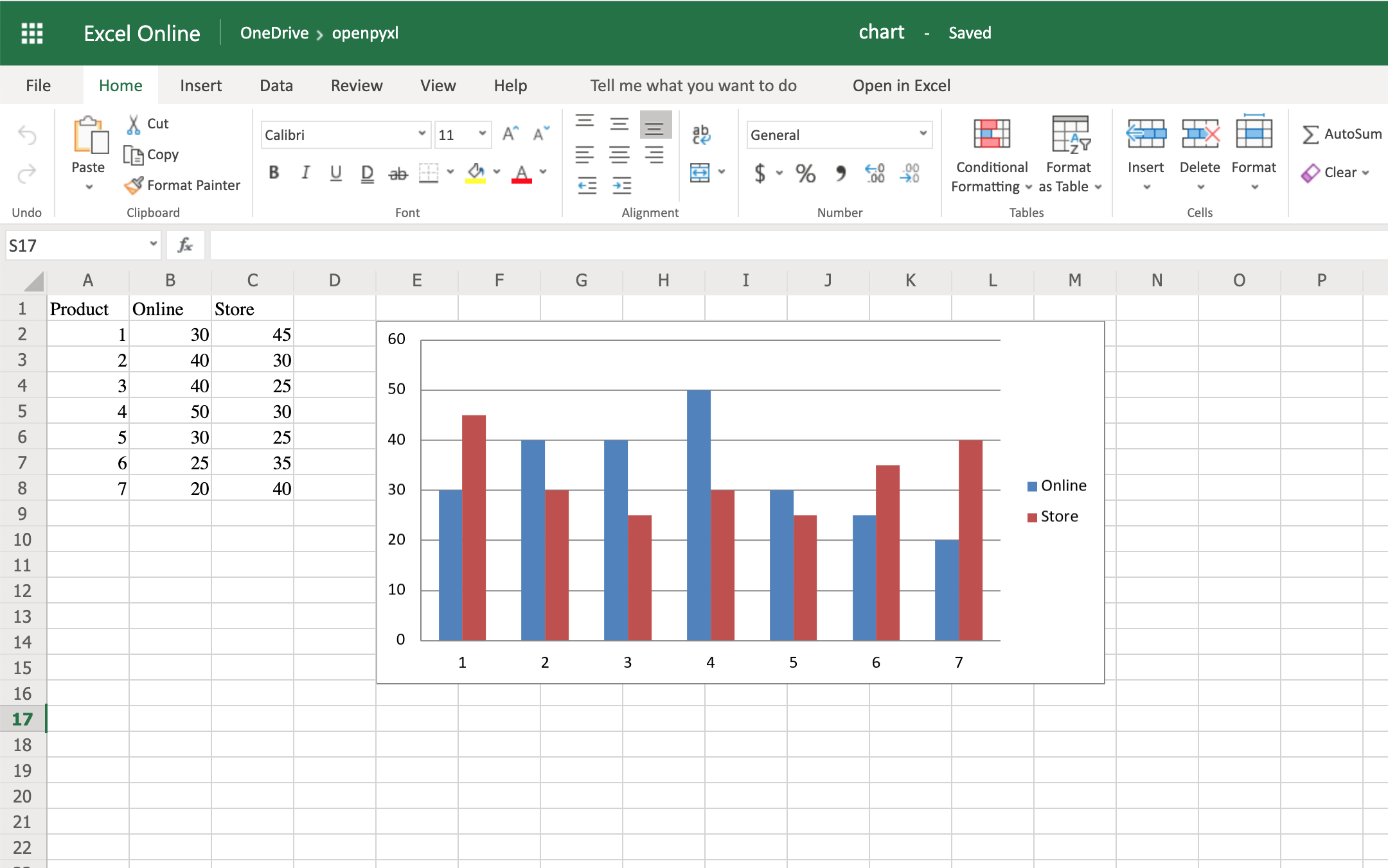 Like with images, the top left corner of the chart is on the cell you added the chart to.
In your case, it was on cell E2.
Note: Depending on whether you're using Microsoft Excel or an open-source alternative (LibreOffice or OpenOffice), the chart might look slightly different.
Try creating a line chart instead, changing the data a bit:
1import random
2from openpyxl import Workbook
3from openpyxl.chart import LineChart, Reference
4
5workbook = Workbook()
6sheet = workbook.active
7
8# Let's create some sample sales data
9rows = [
10 ["", "January", "February", "March", "April",
11 "May", "June", "July", "August", "September",
12 "October", "November", "December"],
13 [1, ],
14 [2, ],
15 [3, ],
16]
17
18for row in rows:
19 sheet.append(row)
20
21for row in sheet.iter_rows(min_row=2,
22 max_row=4,
23 min_col=2,
24 max_col=13):
25 for cell in row:
26 cell.value = random.randrange(5, 100)
With the above code, you'll be able to generate some random data regarding the sales of 3 different products across a whole year.
Once that's done, you can very easily create a line chart with the following code:
28chart = LineChart()
29data = Reference(worksheet=sheet,
30 min_row=2,
31 max_row=4,
32 min_col=1,
33 max_col=13)
34
35chart.add_data(data, from_rows=True, titles_from_data=True)
36sheet.add_chart(chart, "C6")
37
38workbook.save("line_chart.xlsx")
Here's the outcome of the above piece of code:
Like with images, the top left corner of the chart is on the cell you added the chart to.
In your case, it was on cell E2.
Note: Depending on whether you're using Microsoft Excel or an open-source alternative (LibreOffice or OpenOffice), the chart might look slightly different.
Try creating a line chart instead, changing the data a bit:
1import random
2from openpyxl import Workbook
3from openpyxl.chart import LineChart, Reference
4
5workbook = Workbook()
6sheet = workbook.active
7
8# Let's create some sample sales data
9rows = [
10 ["", "January", "February", "March", "April",
11 "May", "June", "July", "August", "September",
12 "October", "November", "December"],
13 [1, ],
14 [2, ],
15 [3, ],
16]
17
18for row in rows:
19 sheet.append(row)
20
21for row in sheet.iter_rows(min_row=2,
22 max_row=4,
23 min_col=2,
24 max_col=13):
25 for cell in row:
26 cell.value = random.randrange(5, 100)
With the above code, you'll be able to generate some random data regarding the sales of 3 different products across a whole year.
Once that's done, you can very easily create a line chart with the following code:
28chart = LineChart()
29data = Reference(worksheet=sheet,
30 min_row=2,
31 max_row=4,
32 min_col=1,
33 max_col=13)
34
35chart.add_data(data, from_rows=True, titles_from_data=True)
36sheet.add_chart(chart, "C6")
37
38workbook.save("line_chart.xlsx")
Here's the outcome of the above piece of code:
 One thing to keep in mind here is the fact that you're using from_rows=True when adding the data.
This argument makes the chart plot row by row instead of column by column.
In your sample data, you see that each product has a row with 12 values (1 column per month).
That's why you use from_rows.
If you don't pass that argument, by default, the chart tries to plot by column, and you'll get a month-by-month comparison of sales.
Another difference that has to do with the above argument change is the fact that our Reference now starts from the first column, min_col=1, instead of the second one.
This change is needed because the chart now expects the first column to have the titles.
There are a couple of other things you can also change regarding the style of the chart.
For example, you can add specific categories to the chart:
cats = Reference(worksheet=sheet,
min_row=1,
max_row=1,
min_col=2,
max_col=13)
chart.set_categories(cats)
Add this piece of code before saving the workbook, and you should see the month names appearing instead of numbers:
One thing to keep in mind here is the fact that you're using from_rows=True when adding the data.
This argument makes the chart plot row by row instead of column by column.
In your sample data, you see that each product has a row with 12 values (1 column per month).
That's why you use from_rows.
If you don't pass that argument, by default, the chart tries to plot by column, and you'll get a month-by-month comparison of sales.
Another difference that has to do with the above argument change is the fact that our Reference now starts from the first column, min_col=1, instead of the second one.
This change is needed because the chart now expects the first column to have the titles.
There are a couple of other things you can also change regarding the style of the chart.
For example, you can add specific categories to the chart:
cats = Reference(worksheet=sheet,
min_row=1,
max_row=1,
min_col=2,
max_col=13)
chart.set_categories(cats)
Add this piece of code before saving the workbook, and you should see the month names appearing instead of numbers:
 Code-wise, this is a minimal change.
But in terms of the readability of the spreadsheet, this makes it much easier for someone to open the spreadsheet and understand the chart straight away.
Another thing you can do to improve the chart readability is to add an axis.
You can do it using the attributes x_axis and y_axis:
chart.x_axis.title = "Months"
chart.y_axis.title = "Sales (per unit)"
This will generate a spreadsheet like the below one:
Code-wise, this is a minimal change.
But in terms of the readability of the spreadsheet, this makes it much easier for someone to open the spreadsheet and understand the chart straight away.
Another thing you can do to improve the chart readability is to add an axis.
You can do it using the attributes x_axis and y_axis:
chart.x_axis.title = "Months"
chart.y_axis.title = "Sales (per unit)"
This will generate a spreadsheet like the below one:
 As you can see, small changes like the above make reading your chart a much easier and quicker task.
There is also a way to style your chart by using Excel's default ChartStyle property.
In this case, you have to choose a number between 1 and 48.
Depending on your choice, the colors of your chart change as well:
# You can play with this by choosing any number between 1 and 48
chart.style = 24
With the style selected above, all lines have some shade of orange:
As you can see, small changes like the above make reading your chart a much easier and quicker task.
There is also a way to style your chart by using Excel's default ChartStyle property.
In this case, you have to choose a number between 1 and 48.
Depending on your choice, the colors of your chart change as well:
# You can play with this by choosing any number between 1 and 48
chart.style = 24
With the style selected above, all lines have some shade of orange:
 There is no clear documentation on what each style number looks like, but this spreadsheet has a few examples of the styles available.
Here's the full code used to generate the line chart with categories, axis titles, and style:
import random
from openpyxl import Workbook
from openpyxl.chart import LineChart, Reference
workbook = Workbook()
sheet = workbook.active
# Let's create some sample sales data
rows = [
["", "January", "February", "March", "April",
"May", "June", "July", "August", "September",
"October", "November", "December"],
[1, ],
[2, ],
[3, ],
]
for row in rows:
sheet.append(row)
for row in sheet.iter_rows(min_row=2,
max_row=4,
min_col=2,
max_col=13):
for cell in row:
cell.value = random.randrange(5, 100)
# Create a LineChart and add the main data
chart = LineChart()
data = Reference(worksheet=sheet,
min_row=2,
max_row=4,
min_col=1,
max_col=13)
chart.add_data(data, titles_from_data=True, from_rows=True)
# Add categories to the chart
cats = Reference(worksheet=sheet,
min_row=1,
max_row=1,
min_col=2,
max_col=13)
chart.set_categories(cats)
# Rename the X and Y Axis
chart.x_axis.title = "Months"
chart.y_axis.title = "Sales (per unit)"
# Apply a specific Style
chart.style = 24
# Save!
sheet.add_chart(chart, "C6")
workbook.save("line_chart.xlsx")
There are a lot more chart types and customization you can apply, so be sure to check out the package documentation on this if you need some specific formatting.
There is no clear documentation on what each style number looks like, but this spreadsheet has a few examples of the styles available.
Here's the full code used to generate the line chart with categories, axis titles, and style:
import random
from openpyxl import Workbook
from openpyxl.chart import LineChart, Reference
workbook = Workbook()
sheet = workbook.active
# Let's create some sample sales data
rows = [
["", "January", "February", "March", "April",
"May", "June", "July", "August", "September",
"October", "November", "December"],
[1, ],
[2, ],
[3, ],
]
for row in rows:
sheet.append(row)
for row in sheet.iter_rows(min_row=2,
max_row=4,
min_col=2,
max_col=13):
for cell in row:
cell.value = random.randrange(5, 100)
# Create a LineChart and add the main data
chart = LineChart()
data = Reference(worksheet=sheet,
min_row=2,
max_row=4,
min_col=1,
max_col=13)
chart.add_data(data, titles_from_data=True, from_rows=True)
# Add categories to the chart
cats = Reference(worksheet=sheet,
min_row=1,
max_row=1,
min_col=2,
max_col=13)
chart.set_categories(cats)
# Rename the X and Y Axis
chart.x_axis.title = "Months"
chart.y_axis.title = "Sales (per unit)"
# Apply a specific Style
chart.style = 24
# Save!
sheet.add_chart(chart, "C6")
workbook.save("line_chart.xlsx")
There are a lot more chart types and customization you can apply, so be sure to check out the package documentation on this if you need some specific formatting.
Convert Python Classes to Excel Spreadsheet
You already saw how to convert an Excel spreadsheet's data into Python classes, but now let's do the opposite.
Let's imagine you have a database and are using some Object-Relational Mapping (ORM) to map DB objects into Python classes.
Now, you want to export those same objects into a spreadsheet.
Let's assume the following data classes to represent the data coming from your database regarding product sales:
from dataclasses import dataclass
from typing import List
@dataclass
class Sale:
quantity: int
@dataclass
class Product:
id: str
name: str
sales: List[Sale]
Now, let's generate some random data, assuming the above classes are stored in a db_classes.py file:
1import random
2
3# Ignore these for now.
You'll use them in a sec ;)
4from openpyxl import Workbook
5from openpyxl.chart import LineChart, Reference
6
7from db_classes import Product, Sale
8
9products = []
10
11# Let's create 5 products
12for idx in range(1, 6):
13 sales = []
14
15 # Create 5 months of sales
16 for _ in range(5):
17 sale = Sale(quantity=random.randrange(5, 100))
18 sales.append(sale)
19
20 product = Product(id=str(idx),
21 name="Product %s" % idx,
22 sales=sales)
23 products.append(product)
By running this piece of code, you should get 5 products with 5 months of sales with a random quantity of sales for each month.
Now, to convert this into a spreadsheet, you need to iterate over the data and append it to the spreadsheet:
25workbook = Workbook()
26sheet = workbook.active
27
28# Append column names first
29sheet.append(["Product ID", "Product Name", "Month 1",
30 "Month 2", "Month 3", "Month 4", "Month 5"])
31
32# Append the data
33for product in products:
34 data = [product.id, product.name]
35 for sale in product.sales:
36 data.append(sale.quantity)
37 sheet.append(data)
That's it.
That should allow you to create a spreadsheet with some data coming from your database.
However, why not use some of that cool knowledge you gained recently to add a chart as well to display that data more visually?
All right, then you could probably do something like this:
38chart = LineChart()
39data = Reference(worksheet=sheet,
40 min_row=2,
41 max_row=6,
42 min_col=2,
43 max_col=7)
44
45chart.add_data(data, titles_from_data=True, from_rows=True)
46sheet.add_chart(chart, "B8")
47
48cats = Reference(worksheet=sheet,
49 min_row=1,
50 max_row=1,
51 min_col=3,
52 max_col=7)
53chart.set_categories(cats)
54
55chart.x_axis.title = "Months"
56chart.y_axis.title = "Sales (per unit)"
57
58workbook.save(filename="oop_sample.xlsx")
Now we're talking! Here's a spreadsheet generated from database objects and with a chart and everything:
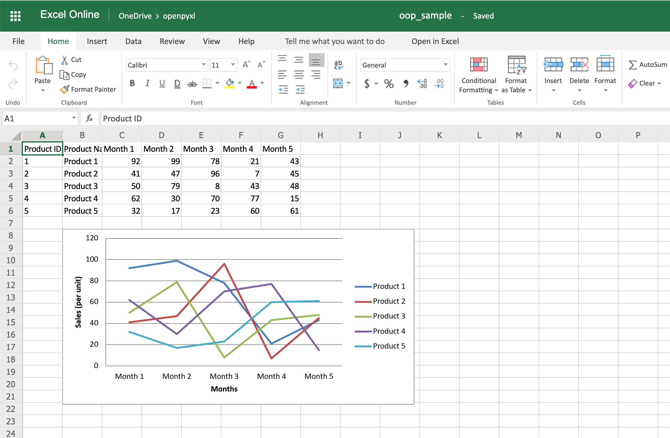 That's a great way for you to wrap up your new knowledge of charts!
Bonus: Working With Pandas
Even though you can use Pandas to handle Excel files, there are few things that you either can't accomplish with Pandas or that you'd be better off just using openpyxl directly.
For example, some of the advantages of using openpyxl are the ability to easily customize your spreadsheet with styles, conditional formatting, and such.
But guess what, you don't have to worry about picking.
In fact, openpyxl has support for both converting data from a Pandas DataFrame into a workbook or the opposite, converting an openpyxl workbook into a Pandas DataFrame.
Note: If you're new to Pandas, check our course on Pandas DataFrames beforehand.
First things first, remember to install the pandas package:
$ pip install pandas
Then, let's create a sample DataFrame:
1import pandas as pd
2
3data = {
4 "Product Name": ["Product 1", "Product 2"],
5 "Sales Month 1": [10, 20],
6 "Sales Month 2": [5, 35],
7}
8df = pd.DataFrame(data)
Now that you have some data, you can use .dataframe_to_rows() to convert it from a DataFrame into a worksheet:
10from openpyxl import Workbook
11from openpyxl.utils.dataframe import dataframe_to_rows
12
13workbook = Workbook()
14sheet = workbook.active
15
16for row in dataframe_to_rows(df, index=False, header=True):
17 sheet.append(row)
18
19workbook.save("pandas.xlsx")
You should see a spreadsheet that looks like this:
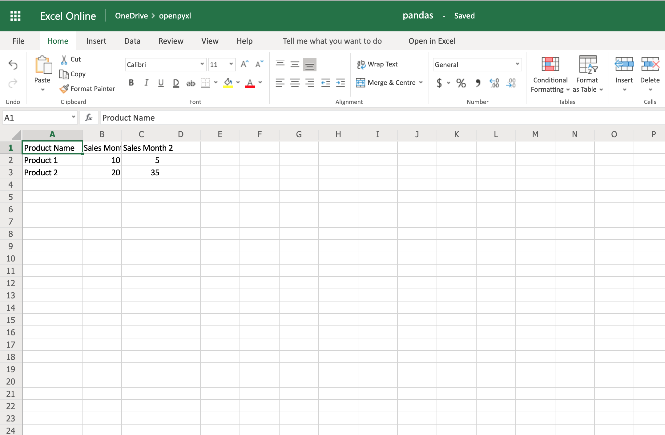 If you want to add the DataFrame's index, you can change index=True, and it adds each row's index into your spreadsheet.
On the other hand, if you want to convert a spreadsheet into a DataFrame, you can also do it in a very straightforward way like so:
import pandas as pd
from openpyxl import load_workbook
workbook = load_workbook(filename="sample.xlsx")
sheet = workbook.active
values = sheet.values
df = pd.DataFrame(values)
Alternatively, if you want to add the correct headers and use the review ID as the index, for example, then you can also do it like this instead:
import pandas as pd
from openpyxl import load_workbook
from mapping import REVIEW_ID
workbook = load_workbook(filename="sample.xlsx")
sheet = workbook.active
data = sheet.values
# Set the first row as the columns for the DataFrame
cols = next(data)
data = list(data)
# Set the field "review_id" as the indexes for each row
idx = [row[REVIEW_ID] for row in data]
df = pd.DataFrame(data, index=idx, columns=cols)
Using indexes and columns allows you to access data from your DataFrame easily:
>>>
>>> df.columns
Index(['marketplace', 'customer_id', 'review_id', 'product_id',
'product_parent', 'product_title', 'product_category', 'star_rating',
'helpful_votes', 'total_votes', 'vine', 'verified_purchase',
'review_headline', 'review_body', 'review_date'],
dtype='object')
>>> # Get first 10 reviews' star rating
>>> df["star_rating"][:10]
R3O9SGZBVQBV76 5
RKH8BNC3L5DLF 5
R2HLE8WKZSU3NL 2
R31U3UH5AZ42LL 5
R2SV659OUJ945Y 4
RA51CP8TR5A2L 5
RB2Q7DLDN6TH6 5
R2RHFJV0UYBK3Y 1
R2Z6JOQ94LFHEP 5
RX27XIIWY5JPB 4
Name: star_rating, dtype: int64
>>> # Grab review with id "R2EQL1V1L6E0C9", using the index
>>> df.loc["R2EQL1V1L6E0C9"]
marketplace US
customer_id 15305006
review_id R2EQL1V1L6E0C9
product_id B004LURNO6
product_parent 892860326
review_headline Five Stars
review_body Love it
review_date 2015-08-31
Name: R2EQL1V1L6E0C9, dtype: object
There you go, whether you want to use openpyxl to prettify your Pandas dataset or use Pandas to do some hardcore algebra, you now know how to switch between both packages.
If you want to add the DataFrame's index, you can change index=True, and it adds each row's index into your spreadsheet.
On the other hand, if you want to convert a spreadsheet into a DataFrame, you can also do it in a very straightforward way like so:
import pandas as pd
from openpyxl import load_workbook
workbook = load_workbook(filename="sample.xlsx")
sheet = workbook.active
values = sheet.values
df = pd.DataFrame(values)
Alternatively, if you want to add the correct headers and use the review ID as the index, for example, then you can also do it like this instead:
import pandas as pd
from openpyxl import load_workbook
from mapping import REVIEW_ID
workbook = load_workbook(filename="sample.xlsx")
sheet = workbook.active
data = sheet.values
# Set the first row as the columns for the DataFrame
cols = next(data)
data = list(data)
# Set the field "review_id" as the indexes for each row
idx = [row[REVIEW_ID] for row in data]
df = pd.DataFrame(data, index=idx, columns=cols)
Using indexes and columns allows you to access data from your DataFrame easily:
>>>
>>> df.columns
Index(['marketplace', 'customer_id', 'review_id', 'product_id',
'product_parent', 'product_title', 'product_category', 'star_rating',
'helpful_votes', 'total_votes', 'vine', 'verified_purchase',
'review_headline', 'review_body', 'review_date'],
dtype='object')
>>> # Get first 10 reviews' star rating
>>> df["star_rating"][:10]
R3O9SGZBVQBV76 5
RKH8BNC3L5DLF 5
R2HLE8WKZSU3NL 2
R31U3UH5AZ42LL 5
R2SV659OUJ945Y 4
RA51CP8TR5A2L 5
RB2Q7DLDN6TH6 5
R2RHFJV0UYBK3Y 1
R2Z6JOQ94LFHEP 5
RX27XIIWY5JPB 4
Name: star_rating, dtype: int64
>>> # Grab review with id "R2EQL1V1L6E0C9", using the index
>>> df.loc["R2EQL1V1L6E0C9"]
marketplace US
customer_id 15305006
review_id R2EQL1V1L6E0C9
product_id B004LURNO6
product_parent 892860326
review_headline Five Stars
review_body Love it
review_date 2015-08-31
Name: R2EQL1V1L6E0C9, dtype: object
There you go, whether you want to use openpyxl to prettify your Pandas dataset or use Pandas to do some hardcore algebra, you now know how to switch between both packages.
run Python script in HTML
run a Python file using HTML using PHP.
Add a PHP file as index.php:
<html>
<head>
<title>Run my Python files</title>
<?PHP
echo shell_exec("python test.py 'parameter1'");
?>
</head>
Passing the parameter to Python
Create a Python file as test.py:
import sys
input=sys.argv[1]
print(input)
Print the parameter passed by PHP.
OHLC Charts in Python
import plotly.graph_objects as go
import pandas as pd
df = pd.read_csv('https://raw.githubusercontent.com/plotly/datasets/master/finance-charts-apple.csv')
fig = go.Figure(data=go.Ohlc(x=df['Date'],
open=df['AAPL.Open'],
high=df['AAPL.High'],
low=df['AAPL.Low'],
close=df['AAPL.Close']))
fig.show()
execute a script within the Python interpreter
exec(open("test.py").read())
PaddleOCR
1.先决条件
确保您的计算机上安装了以下必要先决条件:
Python(3.6 或更高版本)
PaddleOCR 库
其他必要的依赖项(例如 NumPy、pandas 等)
您可以使用以下 pip 命令安装 PaddleOCR:
pip install paddleocr
2.设置 PaddleOCR 一旦您安装了 Python 和所需的库,我们来设置 PaddleOCR。
您可以使用 PaddleOCR 的预训练模型,这些模型可用于文本检测和识别。
代码概览 使用 PaddleOCR 进行文本检测和识别的代码片段包括以下主要组件:
图像预处理:
加载输入图像并执行必要的预处理步骤,例如调整大小或归一化。
文本检测:
使用 PaddleOCR 文本检测模型来定位输入图像中文本区域的边界框。
文本识别:
对于每个检测到的边界框,使用 PaddleOCR 文本识别模型来提取相应的文本。
后处理:
整理检测到的文本和识别结果以进行进一步分析或显示。
3.逐步实现 让我们分解代码片段,详细解释每个步骤:
文本检测 该代码是一个名为 DecMain 的类的一部分,该类专为使用真实数据进行光学字符识别(OCR)评估而设计。
它使用 PaddleOCR 从图像中提取文本,然后计算指标(如准确率、召回率和字符错误率 [CER])来评估 OCR 系统的性能。
class DecMain:
def __init__(self, image_folder_path, label_file_path, output_file):
self.image_folder_path = image_folder_path
self.label_file_path = label_file_path
self.output_file = output_file
def run_dec(self):
# Check and update the ground truth file
CheckAndUpdateGroundTruth(self.label_file_path).check_and_update_ground_truth_file()
df = OcrToDf(image_folder=self.image_folder_path, label_file=self.label_file_path, det=True, rec=True, cls=False).ocr_to_df()
ground_truth_data = ReadGroundTruthFile(self.label_file_path).read_ground_truth_file()
# Get the extracted text as a list of dictionaries (representing the OCR results)
ocr_results = df.to_dict(orient="records")
# Calculate precision, recall, and CER
precision, recall, total_samples = CalculateMetrics(ground_truth_data, ocr_results).calculate_precision_recall()
CreateSheet(dataframe=df, precision=precision, recall=recall, total_samples=total_samples, file_name=self.output_file).create_sheet()
让我们分解代码并解释每个部分:
class DecMain:
def __init__(self, image_folder_path, label_file_path, output_file):
self.image_folder_path = image_folder_path
self.label_file_path = label_file_path
self.output_file = output_file
DecMain 类有一个 __init__方法,用以下参数初始化对象:
image_folder_path:
用于 OCR 的输入图像所在文件夹的路径。
label_file_path:
包含图像的实际文本内容的真实标签文件的路径。
output_file:
评估结果将保存在的输出文件的文件名。
def run_dec(self):
# Check and update the ground truth file
CheckAndUpdateGroundTruth(self.label_file_path).check_and_update_ground_truth_file()
run_dec方法负责运行 OCR 评估过程。
首先,它使用 CheckAndUpdateGroundTruth 类来检查并更新真实标签文件。
df = OcrToDf(image_folder=self.image_folder_path, label_file=self.label_file_path, det=True, rec=True, cls=False).ocr_to_df()
OcrToDf 类用于将 OCR 结果转换为 pandas DataFrame(`df`)。
它接受以下参数:
image_folder:
包含 OCR 输入图像的文件夹的路径。
label_file:
真实标签文件的路径。
det=True和 rec=True参数表示 DataFrame 将包含文本检测和识别结果。
ground_truth_data = ReadGroundTruthFile(self.label_file_path).read_ground_truth_file()
ReadGroundTruthFile 类用于读取真实标签文件并将其内容加载到 ground_truth_data变量中。
# Get the extracted text as a list of dictionaries (representing the OCR results)
ocr_results = df.to_dict(orient="records")
从 DataFrame df 中获取的 OCR 结果转换为字典列表(ocr_results),每个字典代表单个图像的 OCR 结果。
# Calculate precision, recall, and CER
precision, recall, total_samples = CalculateMetrics(ground_truth_data, ocr_results).calculate_precision_recall()
CalculateMetrics 类用于计算 OCR 评估指标:
准确率、召回率和评估的总样本数。
该类将真实数据和 OCR 结果作为输入。
CreateSheet(dataframe=df, precision=precision, recall=recall, total_samples=total_samples, file_name=self.output_file).create_sheet()
CreateSheet 类负责创建输出表格(例如 Excel 或 CSV),其中包含评估指标和 OCR 结果。
它接受 DataFrame `df`、准确率、召回率、总样本数和输出文件名作为输入。
总的来说,DecMain 类提供了一种有条理的方式,使用真实数据和 PaddleOCR 的文本检测和识别功能来评估 OCR 模型的性能。
它计算重要的评估指标,并将结果存储在指定的输出文件中,以供进一步分析。
注意:
真实标签文件的格式 要使用 DecMain 类和提供的代码进行 OCR 评估,必须正确格式化真实标签文件。
真实标签文件应采用 JSON 格式,其结构如下所示:
image_name.jpg [{"transcription": "215mm 18", "points": [[199, 6], [357, 6], [357, 33], [199, 33]], "difficult": False, "key_cls": "digits"}, {"transcription": "XZE SA", "points": [[15, 6], [140, 6], [140, 36], [15, 36]], "difficult": False, "key_cls": "text"}]真实标签文件应为 JSON 格式。
文件的每一行代表图像的 OCR 真实标签。
每一行包含图像的文件名,后跟 JSON 对象形式的该图像的 OCR 结果。
JSON 对象应具有以下几点:
"transcription":
图像的真实文本转录。
"points":
表示图像中文本区域边界框坐标的四个点的列表。
"difficult":
一个布尔值,指示文本区域是否难以识别。
"key_cls":
OCR 结果的类别标签,例如 "digits" 或 "text"。
在创建用于准确评估 OCR 模型性能的真实标签文件时,请确保遵循此格式。
文本识别 代码定义了一个名为 RecMain 的类,该类旨在使用预训练的 OCR 模型在图像文件夹上运行文本识别(OCR)并生成一个评估 Excel 表格。
class RecMain:
def __init__(self, image_folder, rec_file, output_file):
self.image_folder = image_folder
self.rec_file = rec_file
self.output_file = output_file
def run_rec(self):
image_paths = GetImagePathsFromFolder(self.image_folder, self.rec_file).\get_image_paths_from_folder()
ocr_model = LoadRecModel().load_model()
results = ProcessImages(ocr=ocr_model, image_paths=image_paths).process_images()
ground_truth_data = ConvertTextToDict(self.rec_file).convert_txt_to_dict()
model_predictions, ground_truth_texts, image_names, precision, recall, \
overall_model_precision, overall_model_recall, cer_data_list = EvaluateRecModel(results, ground_truth_data).evaluate_model()
# Create Excel sheet
CreateMetricExcel(image_names, model_predictions, ground_truth_texts, precision, recall, cer_data_list, overall_model_precision, overall_model_recall, self.output_file).create_excel_sheet()
让我们分解代码并解释每个部分:
class RecMain:
def __init__(self, image_folder, rec_file, output_file):
self.image_folder = image_folder
self.rec_file = rec_file
self.output_file = output_file
RecMain类有一个__init__方法,用以下参数初始化对象:
image_folder: 包含用于文本识别的输入图像的文件夹路径。
rec_file: 包含图像实际文本内容的地面真实标签文件的路径。
output_file: 保存评估结果的输出Excel表格的文件名。
def run_rec(self):
image_paths = GetImagePathsFromFolder(self.image_folder, self.rec_file).get_image_paths_from_folder()
run_rec方法负责运行文本识别过程。
它首先使用GetImagePathsFromFolder类来获取指定image_folder内所有图像的图像路径列表。
这一步确保OCR模型将处理给定目录内的所有图像。
ocr_model = LoadRecModel().load_model()
LoadRecModel类用于加载用于文本识别的预训练OCR模型。
它可能使用PaddleOCR或其他OCR库来加载模型。
results = ProcessImages(ocr=ocr_model, image_paths=image_paths).process_images()
ProcessImages类负责使用加载的OCR模型来处理图像。
它以OCR模型(ocr_model)和图像路径列表(image_paths)作为输入。
ground_truth_data = ConvertTextToDict(self.rec_file).convert_txt_to_dict()
ConvertTextToDict类用于读取地面实况标签文件并将其转换为字典格式(ground_truth_data)。
这一转换准备了地面实况数据,以便与OCR模型的预测进行比较。
model_predictions, ground_truth_texts, image_names, precision, recall, \
overall_model_precision, overall_model_recall, cer_data_list = EvaluateRecModel(results, ground_truth_data).evaluate_model()
EvaluateRecModel类负责将OCR模型的预测与地面实况数据进行比较,并计算评估指标,如精度、召回率和字符错误率(CER)。
它以OCR模型的预测(results)和地面实况数据(ground_truth_data)作为输入。
# Create Excel sheet
CreateMetricExcel(image_names, model_predictions, ground_truth_texts, precision, recall, cer_data_list, overall_model_precision, overall_model_recall, self.output_file).create_excel_sheet()
CreateMetricExcel类负责创建包含评估指标和OCR结果的输出Excel表。
它接受各种输入数据,包括图像名称、模型预测、地面实况文本、评估指标和输出文件名(self.output_file)。
总之,RecMain类组织了整个文本识别过程,从加载OCR模型到生成包含详细指标的评估Excel表。
它提供了一种有组织和可重复使用的方法,用于评估OCR模型在给定一组图像上的性能。
注:
地面实况文本文件格式使用RecMain类和提供的代码进行OCR评估时,正确格式化地面实况(GT)文本文件至关重要。
GT文本文件应采用以下格式:
image_name.jpg text文件的每一行表示一个图像的GT文本。
每一行包含图像的文件名,后跟一个制表符(\t),然后是该图像的GT文本。
确保GT文本文件包含图像文件夹中指定的所有图像的GT文本条目。
GT文本应与图像中实际文本内容相匹配。
这种格式对于准确评估OCR模型的性能是必需的。
您可以在这里找到源代码:
https://github.com/vinodbaste/paddleOCR_rec_dec?source=post_page结论 我们探讨了如何使用基于深度学习的PaddleOCR进行文本检测和识别的过程。
我们逐步演示了文本检测和识别的实现。
有了PaddleOCR强大的预训练模型和易于使用的API,对图像执行OCR变得更加容易。
微信爬虫Wechat_Articles_Spider
wechat_articles_spider是一个用于爬取微信公众号文章的开源Python工具。
wechat_articles_spider具有以下特点:
自动化爬取:
它能够自动化地从指定的微信公众号中抓取文章数据,省去了手动复制粘贴的繁琐过程。
多线程支持:
该工具支持多线程操作,可以同时处理多个公众号,提高了爬取效率。
高度可定制化:
用户可以根据自己的需求,配置爬取的范围、时间间隔、存储格式等参数,以满足不同的应用场景。
数据持久化:
爬取的文章数据可以方便地保存到本地或数据库中,供后续分析和使用。
安装和使用方法
步骤 1:确保您的系统已安装Python环境,并且具备pip包管理工具。
步骤 2:打开终端或命令提示符,并执行以下命令安装wechat_articles_spider:
pip install wechatarticles
步骤 3:安装完成后,您可以通过导入wechat_articles_spider模块来使用该工具:
import wechat_articles_spider
示例代码
下面是一个简单的示例代码,演示如何使用wechat_articles_spider来爬取微信公众号文章:
import wechat_articles_spider
# 创建一个爬虫实例
spider = wechat_articles_spider.WechatSpider()
# 设置要爬取的公众号名称
spider.set_official_account("公众号名称")
# 设置爬取的文章数量
spider.set_article_count(10)
# 开始爬取文章
spider.start()
# 获取爬取结果
articles = spider.get_articles()
# 打印文章标题和链接
for article in articles:
print("标题:", article['title'])
print("链接:", article['url'])
应用场景
wechat_articles_spider可以应用于多种场景,包括但不限于:
数据分析和挖掘:通过爬取微信公众号文章,可以获取大量的文本数据,用于进行数据分析、情感分析、关键词提取等任务。
新闻媒体监测:可以用于监测特定公众号的文章更新情况,及时获取相关新闻信息。
优缺点
优点:
简单易用,提供了丰富的功能和配置选项。
高效快速,支持多线程操作,提高了爬取效率。
可定制化,用户可以根据需求自定义爬取范围和参数设置。
缺点:
依赖于微信公众号的网页结构,如果微信公众号的页面结构发生变化,可能需要对代码进行适配。
使用该工具需要遵守相关法律法规和网站的使用规则,避免滥用和侵犯他人权益。
two independent programs to communicate with each other
The best way for two independent programs to communicate with each other depends on the specific use case and requirements of the programs.
Both reading and writing to a file and using a local TCP connection are common methods for inter-process communication.
Reading and writing to a file can be a simple and effective way to share data between programs.
However, it may not be the best option for real-time communication or when large amounts of data need to be exchanged frequently.
Using a local TCP connection can provide more real-time communication and can handle larger amounts of data.
However, it requires more setup and configuration, and may not be necessary for simpler communication needs.
Both methods are commonly used in inter-process communication.
To use a local TCP connection for communication between two independent programs, you need to follow these general steps:
Establish a TCP server in one program:
Choose one of the programs to act as the server that will listen for incoming connections.
Create a TCP socket in the server program and bind it to a specific port.
The port number can be any available port that is not already in use.
Here's an example of how to set up a TCP server in Python:
python
import socket
# Create a TCP socket
server_socket = socket.socket(socket.AF_INET, socket.SOCK_STREAM)
# Bind the socket to a specific address and port
server_address = ('localhost', 5000) # Replace 'localhost' with the server's IP address if needed
server_socket.bind(server_address)
# Listen for incoming connections
server_socket.listen(1)
# Accept a client connection
client_socket, client_address = server_socket.accept()
# Now the server is ready to communicate with the client
Connect the TCP client to the server:
In the other program, create a TCP socket and connect it to the server's IP address and port.
Once the connection is established, the client program can send and receive data to/from the server.
Here's an example of how the client program can send and receive data to/from the server using the local TCP connection:
python
import socket
# Create a TCP socket
client_socket = socket.socket(socket.AF_INET, socket.SOCK_STREAM)
# Connect to the server
server_address = ('localhost', 5000) # Replace 'localhost' with the server's IP address if needed
client_socket.connect(server_address)
# Send data to the server
data_to_send = "Hello, server!"
client_socket.sendall(data_to_send.encode())
# Receive data from the server
received_data = client_socket.recv(1024).decode()
print("Received data from server:", received_data)
# Close the connection
client_socket.close()
In this example, the client program creates a TCP socket, connects to the server's IP address and port, and sends data to the server using the sendall() method after encoding the data as bytes.
It then waits to receive a response from the server using the recv() method, specifying the maximum number of bytes to receive (1024 in this case).
The received data is decoded from bytes to a string and printed.
On the server side, you can use a similar approach to receive data from the client and send a response back.
Remember to replace 'localhost' with the appropriate IP address if the server is running on a different machine.
Additionally, you can add exception handling to gracefully handle errors during the connection and communication process.
Here's an example of how the server can receive data from the client and send a response back using the local TCP connection:
python
import socket
# Create a TCP socket
server_socket = socket.socket(socket.AF_INET, socket.SOCK_STREAM)
# Bind the socket to a specific address and port
server_address = ('localhost', 5000) # Replace 'localhost' with the server's IP address if needed
server_socket.bind(server_address)
# Listen for incoming connections
server_socket.listen(1)
# Accept a client connection
client_socket, client_address = server_socket.accept()
# Receive data from the client
received_data = client_socket.recv(1024).decode()
print("Received data from client:", received_data)
# Process the received data (e.g., perform calculations, generate a response)
# Send a response back to the client
response_data = "Hello, client!"
client_socket.sendall(response_data.encode())
# Close the connection
client_socket.close()
server_socket.close()
In this example, after accepting the client connection, the server program waits to receive data from the client using the recv() method, specifying the maximum number of bytes to receive (1024 in this case).
The received data is then decoded from bytes to a string and processed as needed. In this case, we simply generate a response message.
After processing the data and generating a response, the server uses the sendall() method to send the response back to the client.
The response data is encoded as bytes before sending.
Finally, the server and client sockets are closed to release the resources and terminate the connection.
Remember to replace 'localhost' with the appropriate IP address if the server is running on a different machine. Similarly, you can add exception handling to handle errors gracefully during the connection and communication process.
使用Python读取日期和时间
可以使用内置的文件操作功能和日期时间处理模块。
import datetime
# 读取闹钟日期和时间的文本文件路径
file_path = "path/to/alarms.txt"
# 存储闹钟日期和时间的列表
alarms = []
# 打开文本文件并读取闹钟日期和时间
with open(file_path, "r") as file:
for line in file:
alarm = line.strip()
alarms.append(alarm)
# 处理每个闹钟
for alarm in alarms:
# 获取当前日期和时间
current_datetime = datetime.datetime.now()
alarm_datetime = datetime.datetime.strptime(alarm, "%Y-%m-%d %H:%M:%S")
# 计算下一个闹钟日期和时间
if alarm_datetime < current_datetime:
next_alarm = alarm_datetime + datetime.timedelta(days=1)
else:
next_alarm = alarm_datetime
# 计算闹钟触发时间间隔(秒)
interval = (next_alarm - current_datetime).total_seconds()
# 等待时间间隔并触发闹钟
import time
time.sleep(interval)
print("闹钟日期和时间:", alarm)
print("闹钟响铃!")
在这个示例代码中,您需要将 file_path 变量设置为包含闹钟日期和时间的文本文件的路径。
代码将打开文件并逐行读取闹钟的日期和时间,然后将其存储在 alarms 列表中。
每个闹钟的日期和时间应以 "YYYY-MM-DD HH:MM:SS" 的格式存储在文本文件中,每行一个闹钟。
代码处理每个闹钟,计算下一个闹钟日期和时间,并使用 time.sleep 函数等待时间间隔,然后触发闹钟。
在示例代码中,我使用 print 语句来显示闹钟日期和时间以及响铃提醒,您可以根据需要进行调整。
Python内置数据库:SQLite
import sqlite3
# 连接到数据库
conn = sqlite3.connect('example.db')
# 创建一个游标对象
cursor = conn.cursor()
# 执行一个查询
cursor.execute('SELECT SQLITE_VERSION()')
# 打印查询结果
data = cursor.fetchone()
print("SQLite version:", data)
# SQLite version: ('3.40.1',)
# 创建表格
# 创建一个名为students的表,包含id、name和age三个字段
cursor.execute('''CREATE TABLE students (id INTEGER PRIMARY KEY, name TEXT, age INTEGER)''')
# cursor.execute('''CREATE TABLE stocks
# (date text, trans text, symbol text, qty real, price real)''')
# 插入数据
# 向students表中插入一条数据
cursor.execute("INSERT INTO students (name, age) VALUES ('张三', 20)")
# cursor.execute("INSERT INTO stocks VALUES ('2022-10-28', 'BUY', 'GOOG', 100, 490.1)")
# 保存更改
conn.commit()
# 查询users表中的所有数据
cursor.execute("SELECT * FROM students")
rows = cursor.fetchall()
# 打印查询结果
for row in rows:
print(row)
# 更新users表中id为1的数据的name字段为'李四'
cursor.execute("UPDATE students SET name=? WHERE id=?", ('李四', 1))
# 查询users表中的所有数据
cursor.execute("SELECT * FROM students")
rows = cursor.fetchall()
# 打印查询结果
for row in rows:
print(row)
# 删除users表中id为1的数据
cursor.execute("DELETE FROM students WHERE id=?", (1,))
# 提交更改并关闭连接
conn.commit()
# 关闭连接
conn.close()
Python SQLite
Python sqlite3 module APIs
Connect To Database
Create a Table
INSERT Operation
SELECT Operation
UPDATE Operation
DELETE Operation
To use sqlite3 module, you must first create a connection object that represents the database and then optionally you can create a cursor object, which will help you in executing all the SQL statements.
Python sqlite3 module APIs
⇧
Following are important sqlite3 module routines, which can suffice your requirement to work with SQLite database from your Python program.
If you are looking for a more sophisticated application, then you can look into Python sqlite3 module's official documentation.
Sr.No. API & Description 1 sqlite3.connect(database [,timeout ,other optional arguments])
This API opens a connection to the SQLite database file.
You can use ":memory:" to open a database connection to a database that resides in RAM instead of on disk.
If database is opened successfully, it returns a connection object.
When a database is accessed by multiple connections, and one of the processes modifies the database, the SQLite database is locked until that transaction is committed.
The timeout parameter specifies how long the connection should wait for the lock to go away until raising an exception.
The default for the timeout parameter is 5.0 (five seconds).
If the given database name does not exist then this call will create the database.
You can specify filename with the required path as well if you want to create a database anywhere else except in the current directory.
2 connection.cursor([cursorClass])
This routine creates a cursor which will be used throughout of your database programming with Python.
This method accepts a single optional parameter cursorClass.
If supplied, this must be a custom cursor class that extends sqlite3.Cursor.
3 cursor.execute(sql [, optional parameters])
This routine executes an SQL statement.
The SQL statement may be parameterized (i.e. placeholders instead of SQL literals).
The sqlite3 module supports two kinds of placeholders: question marks and named placeholders (named style).
For example − cursor.execute("insert into people values (?, ?)", (who, age))4 connection.execute(sql [, optional parameters])
This routine is a shortcut of the above execute method provided by the cursor object and it creates an intermediate cursor object by calling the cursor method, then calls the cursor's execute method with the parameters given.
5 cursor.executemany(sql, seq_of_parameters)
This routine executes an SQL command against all parameter sequences or mappings found in the sequence sql.
6 connection.executemany(sql[, parameters])
This routine is a shortcut that creates an intermediate cursor object by calling the cursor method, then calls the cursor.s executemany method with the parameters given.
7 cursor.executescript(sql_script)
This routine executes multiple SQL statements at once provided in the form of script.
It issues a COMMIT statement first, then executes the SQL script it gets as a parameter.
All the SQL statements should be separated by a semi colon (;).
8 connection.executescript(sql_script)
This routine is a shortcut that creates an intermediate cursor object by calling the cursor method, then calls the cursor's executescript method with the parameters given.
9 connection.total_changes()
This routine returns the total number of database rows that have been modified, inserted, or deleted since the database connection was opened.
10 connection.commit()
This method commits the current transaction.
If you don't call this method, anything you did since the last call to commit() is not visible from other database connections.
11 connection.rollback()
This method rolls back any changes to the database since the last call to commit().
12 connection.close()
This method closes the database connection.
Note that this does not automatically call commit().
If you just close your database connection without calling commit() first, your changes will be lost!
13 cursor.fetchone()
This method fetches the next row of a query result set, returning a single sequence, or None when no more data is available.
14 cursor.fetchmany([size = cursor.arraysize])This routine fetches the next set of rows of a query result, returning a list.
An empty list is returned when no more rows are available.
The method tries to fetch as many rows as indicated by the size parameter.
15 cursor.fetchall()
This routine fetches all (remaining) rows of a query result, returning a list.
An empty list is returned when no rows are available.
Connect To Database
⇧
Following Python code shows how to connect to an existing database.
If the database does not exist, then it will be created and finally a database object will be returned.
#!/usr/bin/python
import sqlite3
conn = sqlite3.connect('test.db')
print "Opened database successfully";
Here, you can also supply database name as the special name :memory: to create a database in RAM.
Now, let's run the above program to create our database test.db in the current directory.
You can change your path as per your requirement.
Keep the above code in sqlite.py file and execute it as shown below.
If the database is successfully created, then it will display the following message.
$chmod +x sqlite.py
$./sqlite.py
Open database successfully
Create a Table
⇧
Following Python program will be used to create a table in the previously created database.
#!/usr/bin/python
import sqlite3
conn = sqlite3.connect('test.db')
print "Opened database successfully";
conn.execute('''CREATE TABLE COMPANY
(ID INT PRIMARY KEY NOT NULL,
NAME TEXT NOT NULL,
AGE INT NOT NULL,
ADDRESS CHAR(50),
SALARY REAL);''')
print "Table created successfully";
conn.close()
When the above program is executed, it will create the COMPANY table in your test.db and it will display the following messages −
Opened database successfully
Table created successfully
INSERT Operation
⇧
Following Python program shows how to create records in the COMPANY table created in the above example.
#!/usr/bin/python
import sqlite3
conn = sqlite3.connect('test.db')
print "Opened database successfully";
conn.execute("INSERT INTO COMPANY (ID,NAME,AGE,ADDRESS,SALARY) \
VALUES (1, 'Paul', 32, 'California', 20000.00 )");
conn.execute("INSERT INTO COMPANY (ID,NAME,AGE,ADDRESS,SALARY) \
VALUES (2, 'Allen', 25, 'Texas', 15000.00 )");
conn.execute("INSERT INTO COMPANY (ID,NAME,AGE,ADDRESS,SALARY) \
VALUES (3, 'Teddy', 23, 'Norway', 20000.00 )");
conn.execute("INSERT INTO COMPANY (ID,NAME,AGE,ADDRESS,SALARY) \
VALUES (4, 'Mark', 25, 'Rich-Mond ', 65000.00 )");
conn.commit()
print "Records created successfully";
conn.close()
When the above program is executed, it will create the given records in the COMPANY table and it will display the following two lines −
Opened database successfully
Records created successfully
SELECT Operation
⇧
Following Python program shows how to fetch and display records from the COMPANY table created in the above example.
#!/usr/bin/python
import sqlite3
conn = sqlite3.connect('test.db')
print "Opened database successfully";
cursor = conn.execute("SELECT id, name, address, salary from COMPANY")
for row in cursor:
print "ID = ", row[0]
print "NAME = ", row[1]
print "ADDRESS = ", row[2]
print "SALARY = ", row[3], "\n"
print "Operation done successfully";
conn.close()
When the above program is executed, it will produce the following result.
Opened database successfully
ID = 1
NAME = Paul
ADDRESS = California
SALARY = 20000.0
ID = 2
NAME = Allen
ADDRESS = Texas
SALARY = 15000.0
ID = 3
NAME = Teddy
ADDRESS = Norway
SALARY = 20000.0
ID = 4
NAME = Mark
ADDRESS = Rich-Mond
SALARY = 65000.0
Operation done successfully
UPDATE Operation
⇧
Following Python code shows how to use UPDATE statement to update any record and then fetch and display the updated records from the COMPANY table.
#!/usr/bin/python
import sqlite3
conn = sqlite3.connect('test.db')
print "Opened database successfully";
conn.execute("UPDATE COMPANY set SALARY = 25000.00 where ID = 1")
conn.commit()
print "Total number of rows updated :", conn.total_changes
cursor = conn.execute("SELECT id, name, address, salary from COMPANY")
for row in cursor:
print "ID = ", row[0]
print "NAME = ", row[1]
print "ADDRESS = ", row[2]
print "SALARY = ", row[3], "\n"
print "Operation done successfully";
conn.close()
When the above program is executed, it will produce the following result.
Opened database successfully
Total number of rows updated : 1
ID = 1
NAME = Paul
ADDRESS = California
SALARY = 25000.0
ID = 2
NAME = Allen
ADDRESS = Texas
SALARY = 15000.0
ID = 3
NAME = Teddy
ADDRESS = Norway
SALARY = 20000.0
ID = 4
NAME = Mark
ADDRESS = Rich-Mond
SALARY = 65000.0
Operation done successfully
DELETE Operation
⇧
Following Python code shows how to use DELETE statement to delete any record and then fetch and display the remaining records from the COMPANY table.
#!/usr/bin/python
import sqlite3
conn = sqlite3.connect('test.db')
print "Opened database successfully";
conn.execute("DELETE from COMPANY where ID = 2;")
conn.commit()
print "Total number of rows deleted :", conn.total_changes
cursor = conn.execute("SELECT id, name, address, salary from COMPANY")
for row in cursor:
print "ID = ", row[0]
print "NAME = ", row[1]
print "ADDRESS = ", row[2]
print "SALARY = ", row[3], "\n"
print "Operation done successfully";
conn.close()
When the above program is executed, it will produce the following result.
Opened database successfully
Total number of rows deleted : 1
ID = 1
NAME = Paul
ADDRESS = California
SALARY = 20000.0
ID = 3
NAME = Teddy
ADDRESS = Norway
SALARY = 20000.0
ID = 4
NAME = Mark
ADDRESS = Rich-Mond
SALARY = 65000.0
Operation done successfully
AI can provide valuable assistance in learning programming
specifically Python, in the following ways:
Interactive Learning Platforms: AI-powered platforms can offer interactive lessons and tutorials for learning Python.
These platforms can provide step-by-step instructions, coding challenges, and interactive coding environments where learners can practice writing and executing Python code.
AI algorithms can analyze learners' code and provide immediate feedback, helping them identify and correct errors.
Intelligent Code Autocompletion: AI-based code editors and integrated development environments (IDEs) can offer intelligent code autocompletion suggestions while programming in Python.
These suggestions are based on context, syntax, and common programming patterns.
AI-powered autocompletion can help learners explore different options, reduce syntax errors, and improve coding efficiency.
Error Detection and Debugging: AI can assist in detecting and debugging errors in Python code.
By analyzing code syntax, structure, and runtime behavior, AI algorithms can identify potential errors, offer suggestions for correction, and provide explanations for common mistakes.
This helps learners understand and resolve coding issues more effectively.
Code Generation and Examples: AI can generate Python code snippets or complete functions based on specified requirements or desired outcomes.
This can be particularly helpful for beginners who are learning the language and need assistance with writing correct and functional code.
AI can also provide real-life examples of Python code usage in various applications and domains.
Natural Language Processing (NLP): AI-powered NLP capabilities can aid in understanding Python documentation, tutorials, and forums.
NLP algorithms can analyze and interpret text-based resources, extract relevant information, and provide explanations in a more accessible and understandable format.
This can assist learners in comprehending complex programming concepts and syntax.
Intelligent Recommendations: AI algorithms can recommend relevant learning resources, tutorials, and projects based on learners' proficiency level, interests, and areas of improvement.
These recommendations can help learners discover additional learning materials, practice Python in different contexts, and explore advanced topics at their own pace.
Collaborative Learning and Coding Communities: AI can facilitate collaborative learning and coding communities by connecting learners with peers, mentors, and experts in Python programming.
AI-powered platforms can match learners with similar interests or skill levels for group projects, coding challenges, and code reviews.
This fosters an environment of peer support, knowledge sharing, and collective learning.
AI-based Python Libraries and Frameworks: AI libraries and frameworks like TensorFlow, PyTorch, and scikit-learn provide powerful tools for developing AI and machine learning applications in Python.
Learning these libraries and frameworks can open up opportunities to explore and apply AI techniques within Python programming.
It's important to note that while AI can assist in learning Python, hands-on practice, active problem-solving, and engagement with programming exercises and projects remain crucial for developing programming skills.
AI serves as a supportive tool to enhance the learning experience, but it should not replace practical coding experience and conceptual understanding.
Here are a few interactive learning platforms that can help you learn Python programming:
Codecademy (www.codecademy.com): Codecademy offers interactive Python courses that guide learners through coding exercises, projects, and quizzes.
The platform provides a hands-on learning experience and covers topics ranging from Python basics to advanced concepts.
Coursera (www.coursera.org): Coursera hosts a variety of Python programming courses offered by universities and institutions worldwide.
These courses often include interactive coding exercises, video lectures, and assignments to reinforce learning.
DataCamp (www.datacamp.com): DataCamp specializes in data science and offers interactive Python courses focused on data analysis, visualization, and machine learning.
The platform provides a learn-by-doing approach with coding exercises and real-world projects.
edX (www.edx.org): edX offers Python courses from renowned universities and institutions.
These courses cover Python fundamentals, web development, data science, and more.
The platform provides interactive coding exercises and assessments to test your knowledge.
SoloLearn (www.sololearn.com): SoloLearn offers a mobile app and web platform with interactive Python courses.
The courses are designed in a gamified format, allowing learners to earn points, compete with peers, and practice coding challenges.
Codewars (www.codewars.com): Codewars provides a platform for users to solve coding challenges in various programming languages, including Python.
You can choose Python-specific challenges of different difficulty levels and learn from community solutions.
JetBrains Academy (www.jetbrains.com/academy): JetBrains Academy offers an interactive learning platform with Python courses and projects.
The platform provides an integrated development environment (IDE) and offers step-by-step guidance for learning Python and building real-world applications.
Remember, while these platforms provide interactive learning experiences, it\'s important to practice coding regularly, work on projects, and engage in problem-solving to solidify your Python programming skills.
create new project process
create dir
cd dir
git init
git remote add origin git@github.com:$USERNAME/$1.git
touch README.md
git add .
git commit -m "Initial commit"
git push -u origin master
code .
Build Android Apps with Flet in Python
Build Android Apps with Flet in Python (APKs)
Pygubu: 快速开发Python tkinter用户界面
pip install pygubu-designer
Pygubu is a RAD tool to enable quick and easy development of user interfaces for the Python's tkinter module.
The user interfaces designed are saved as XML files, and, by using the pygubu builder, these can be loaded by applications dynamically as needed.
https://github.com/alejandroautalan/pygubu-designer
Usage
Type on the terminal the following commands.
C:\Python3\Scripts\pygubu-designer.exe
Where C:\Python3 is the path to your Python installation directory.
wechat
Python 微信自动化操作
用 Python 发送通知到微信
用python控制微信
Python操作微信
Could not install packages due to an OSError:
[WinError 2] No such file or directory
The system cannot find the file specified: 'C:\\Python311\\Scripts\\chardetect.exe' -> 'C:\\Python311\\Scripts\\chardetect.exe.deleteme'
Try running the command as administrator:
or
pip install numpy --user to install numpy without any special previlages
数据分析-主成分分析 (PCA)
主成分分析(Principal Component Analysis, PCA)是一种用于数据降维的统计技术。
它的目的是通过将原始数据转化为一组新的不相关的变量(称为主成分),来减少数据的维度,同时保留数据中最重要的信息。
PCA 的具体步骤
⇧
标准化数据 :
由于不同特征可能具有不同的单位和量级,因此在进行PCA之前,需要对数据进行标准化处理(通常是零均值和单位方差)。
计算协方差矩阵 :
协方差矩阵用于测量数据集中的特征之间的线性相关性。
计算特征值和特征向量 :
协方差矩阵的特征值和特征向量用于确定主成分。
特征值表示主成分解释的数据方差的大小,特征向量则表示主成分的方向。
选择主成分 :
根据特征值的大小排序,选择前k个特征值对应的特征向量作为主成分。
变换数据 :
将原始数据投影到选择的主成分上,得到降维后的数据集。
PCA 适用于以下场景
⇧
降维 :在高维数据集中减少维度,同时保留数据中最重要的信息。
去除噪音 :通过去除解释较少方差的次要成分,减少数据中的噪音。
数据可视化 :将高维数据投影到二维或三维空间中,以便可视化。
特征选择 :识别和选择对数据变异贡献最大的特征。
优点
⇧
降维有效 :能够有效地减少数据的维度,保留主要信息。
去除冗余 :去除特征间的多重共线性,简化模型。
提高计算效率 :降低数据维度,提高后续算法的计算效率。
缺点
⇧
解释性差 :主成分是线性组合,不容易解释原始特征的实际意义。
信息丢失 :降维过程中可能会丢失一些信息,尤其是当保留的主成分数量较少时。
线性假设 :假设特征间的关系是线性的,对于非线性关系效果较差。
注意事项
⇧
数据标准化 :在进行 PCA 之前,一定要对数据进行标准化处理。
特征选择 :选择合适的主成分数量,通常通过累计解释方差来确定。
异常值 :注意数据中的异常值,因为它们可能会对 PCA 结果产生较大影响。
如何找到最优值
⇧
确定最优主成分数量通常通过累计解释方差的方法来进行。
具体步骤如下:
计算每个主成分的解释方差 。
计算累计解释方差 ,并绘制累计解释方差图(即 Scree Plot)。
选择拐点 :通常选择累计解释方差达到 90% 或解释方差显著下降的拐点对应的主成分数量。
实际数据演示
⇧
我们将使用Python模拟一个电商数据集,包含多个维度的数据,然后通过 PCA 进行降维处理,并找出最优解。
首先,我们生成模拟的电商数据,并对其进行标准化处理↓
import numpy as np
import pandas as pd
from sklearn.preprocessing import StandardScaler
np.random.seed(0)
data = {
'customer_id': np.arange(1, 101),
'age': np.random.randint(18, 70, size=100),
'annual_income': np.random.randint(20000, 150000, size=100),
'spending_score': np.random.randint(1, 100, size=100),
'years_as_customer': np.random.randint(1, 10, size=100),
'total_purchases': np.random.randint(1, 50, size=100),
'average_purchase_value': np.random.randint(10, 1000, size=100),
'purchase_frequency': np.random.randint(1, 12, size=100)
}
df = pd.DataFrame(data)
features = df.drop('customer_id', axis=1)
scaler = StandardScaler()
scaled_features = scaler.fit_transform(features)
 接下来,我们对标准化后的数据进行 PCA 分析,并计算累计解释方差。
from sklearn.decomposition import PCA
import matplotlib.pyplot as plt
pca = PCA()
pca_features = pca.fit_transform(scaled_features)
# 计算累计解释方差
explained_variance = np.cumsum(pca.explained_variance_ratio_)
# 绘制 Scree Plot
plt.figure(figsize=(10, 6))
plt.plot(range(1, len(explained_variance) + 1), explained_variance, marker='o', linestyle='--')
plt.title('Scree Plot')
plt.xlabel('Number of Components')
plt.ylabel('Cumulative Explained Variance')
plt.axhline(y=0.9, color='r', linestyle='--')
plt.text(1, 0.85, '90% cut-off threshold', color='red', fontsize=12)
plt.show()
print("Explained Variance Ratios:", pca.explained_variance_ratio_)
print("Cumulative Explained Variance:", explained_variance)
 根据累计解释方差图,我们选择前3个主成分作为最终的降维结果↓
# 选择前3个主成分
pca = PCA(n_components=3)
pca_features = pca.fit_transform(scaled_features)
# 打印每个主成分的解释方差
print("Explained Variance Ratios for 3 Components:", pca.explained_variance_ratio_)
我们可以通过散点图来可视化前两个主成分。
# 可视化前两个主成分
plt.figure(figsize=(10, 6))
sns.scatterplot(x=pca_features[:, 0], y=pca_features[:, 1], hue=df['spending_score'], palette='viridis')
plt.title('PCA - 可视化前两个主成分')
plt.xlabel('主成分-1')
plt.ylabel('主成分-2')
plt.colorbar(label='Spending Score')
plt.show()
 最后,我们对新数据进行标准化处理,并通过 PCA 转换进行降维。
# 新数据预测
new_data = np.array([[25, 45000, 75, 3, 20, 250, 6]])
new_data_scaled = scaler.transform(new_data)
new_data_pca = pca.transform(new_data_scaled)
print(f"New data PCA transformation: {new_data_pca}")
通过上述步骤,我们使用 PCA 对高维电商数据进行了降维处理。
我们详细解释了每一步的过程,并通过累计解释方差图确定了最佳的主成分数量,最后对降维后的数据进行了可视化处理。
同时,我们演示了如何对新数据进行 PCA 转换,以便进行预测。
Download Video in MP3 format using PyTube
Pytube is a lightweight, Python-written library.
Pytube provides a command-line feature that allows you to stream videos directly from the terminal easily.
To import pytube, we can use the commands according to the python version.
For Python2 : pip install pytube
For Python3 : pip3 install pytube
For pyube3 : pip install pytube3
To save the audio file, we are using the os module:
pip install os_sys
Procedure:
First, we need to import the required (pytube and os) module.
Implementation: Python3
# importing packages
from pytube import YouTube
import os
# url input from user
yt = YouTube(
str(input("Enter the URL of the video you want to download: \n>> ")))
# extract only audio
video = yt.streams.filter(only_audio=True).first()
# check for destination to save file
print("Enter the destination (leave blank for current directory)")
destination = str(input(">> ")) or '.'
# download the file
out_file = video.download(output_path=destination)
# save the file
base, ext = os.path.splitext(out_file)
new_file = base + '.mp3'
os.rename(out_file, new_file)
# result of success
print(yt.title + " has been successfully downloaded.")
Cut MP3 file
Before we go forward, we need to install FFmpeg in your system as it is required to deal with mp3 files to download you can visit this site: https://phoenixnap.com/kb/ffmpeg-windows.
Also, we will use pydub library to perform this task.
pip install pydub
Step 1: Open an mp3 file using pydub.
from pydub import AudioSegment
song = AudioSegment.from_mp3("test.mp3")
Step 2: Slice audio
# pydub does things in milliseconds
ten_seconds = 10 * 1000
first_10_seconds = song[:ten_seconds]
last_5_seconds = song[-5000:]
Step 3: Save the results as a new file in mp3 audio format.
first_10_seconds.export("new.mp3", format="mp3")
Example:
from pydub import AudioSegment
# Open an mp3 file
song = AudioSegment.from_file("testing.mp3",
format="mp3")
# pydub does things in milliseconds
ten_seconds = 10 * 1000
# song clip of 10 seconds from starting
first_10_seconds = song[:ten_seconds]
# save file
first_10_seconds.export("first_10_seconds.mp3",
format="mp3")
print("New Audio file is created and saved")
用Python开发音乐爬虫
首先准备
环境
Python 3.10
Pycharm
模块
import requests >>> pip install requests
import parsel >>> pip install parsel
import prettytable >>> pip install prettytable
import os
打包exe程序:
pyinstaller > pip install pyinstaller
文章看的不理解,我还录制了详细的视频讲解,和源码一起打包好了,私信小编,发送关键字【学习】自动掉落
爬虫实现基本流程
案例分为三部分:
单首歌曲采集
搜索下载功能 (单个/批量)
把py程序打包成exe软件
一、数据来源分析
1、明确需求
明确采集的网站以及数据内容
网址: https://www.gequbao.com/music/402856
数据: 歌曲链接
2.抓包分析
通过浏览器开发者工具分析对应的数据位置
打开开发者工具
F12 / 右键点击检查选择network 网络
刷新网页
通过关键字搜索找到对应数据位置
先找歌曲链接地址(播放地址): 开发者工具 > 网络 > 媒体 > 查看对应歌曲链接
再根据链接中一段参数进行搜索
关键字: 需要什么数据就搜什么数据
数据包地址: https://www.gequbao.com/api/play_url?id=402856&json=1
二、代码实现步骤
1.发送请求
模拟浏览器对于url地址发送请求
# 导入数据请求模块 import requests """发送请求"""
# 模拟浏览器 (请求头)
headers = {
# User-Agent 用户代理, 表示浏览器基本身份信息
'User-Agent':'Mozilla/5.0 (Windows NT 10.0; Win64; x64) AppleWebKit/537.36 (KHTML, like Gecko) Chrome/126.0.0.0 Safari/537.36'
}
# 请求网址
url = 'https://www.gequbao.com/api/play_url?id=402856&json=1' # 发送请求
response = requests.get(url=url, headers=headers)
2.获取数据
获取服务器返回响应数据
# 获取响应json数据
json_data = response.json()
3.解析数据
提取我们需要的数据内容
css选择器简单使用
根据标签属性提取数据内容
查看数据对应标签位置
4.保存数据
获取歌曲内容, 保存到本地文件夹
# 对于歌曲链接发送请求, 获取歌曲内容
music_content = requests.get(url=play_url, headers=headers).content
# 数据保存
with open(f'music\\{download_title}-{download_singer}.mp3', mode='wb') as f:
# 写入数据
f.write(music_content)
print(f'{download_title}歌曲下载完成!')
5.搜索下载
找搜索接口
歌名
歌曲ID
分析不同歌曲, 数据包有什么变化
歌曲变化 > ID
只要过去所有歌曲ID你就可以采集所有歌曲内容
效果展示
6.打包EXE
pyinstaller -F xx.py
打包成功后,就能分享给其它不会py的小伙伴,愉快的使用了
自动化地完成各种任务 Python Scripts
项目地址:https://github.com/DhanushNehru/Python-Scripts
部分脚本介绍
•Arrange It: 根据文件扩展名自动将文件移动到相应的文件夹。
•Auto WiFi Check: 监控 WiFi 连接是否正常。
•AutoCert: 批量生成电子证书。
•Automated Emails: 读取 CSV 文件,发送个性化的邮件。
•Black Hat Python: 来自《黑帽子 Python》一书的源代码。
•Blackjack: 一个二十一点游戏。
•Chessboard: 使用 matplotlib 创建一个棋盘。
•Compound Interest Calculator: 一个计算复利的 Python 脚本。
•Countdown Timer: 当输入的时间过去时显示一条消息。
•Convert Temperature: 一个 Python 脚本,用于在华氏度、摄氏度和开氏度之间转换温度。
•Crop Images: 一个 Python 脚本,用于裁剪给定的图像。
•CSV to Excel: 一个 Python 脚本,用于将 CSV 文件转换为 Excel 文件。
•Currency Script: 一个 Python 脚本,用于将一个国家的货币转换为另一个国家的货币。
•Digital Clock: 一个 Python 脚本,用于在终端中显示一个数字时钟。
•Display Popup Window: 一个 Python 脚本,用于向用户预览一个 GUI 界面。
•Duplicate Finder: 该脚本通过 MD5 哈希识别重复文件,并允许删除或重新定位文件。
•Emoji in PDF: 一个 Python 脚本,用于在 PDF 中查看 Emoji。
•Expense Tracker: 一个 Python 脚本,可以跟踪开支。
•Face Reaction: 一个试图检测面部表情的脚本。
•Fake Profiles: 创建虚假配置文件。
•File Encryption Decryption: 使用 AES 算法对文件进行加密和解密,以确保安全性。
•Font Art: 使用 Python 显示字体艺术。
•Freelance Helper Program: 从包含工作时间的 Excel 文件中获取数据,并计算报酬。
•Get Hexcodes From Websites: 从网站生成包含十六进制代码的 Python 列表。
•Hand_Volume: 检测和跟踪手部动作,以控制音量。
•Harvest Predictor: 接收一些必要的输入参数,并根据这些参数预测收成。
•Html-to-images: 将 HTML 文档转换为图像文件。
•Image Capture: 从网络摄像头捕捉图像并将其保存到本地设备。
•Image Compress: 压缩图像。
•Image Manipulation without libraries: 在不使用任何外部库的情况下,操作图像。
•Image Text: 从图像中提取文本。
•Image Text to PDF: 将图像和文本添加到 PDF 文件中。
•Image Watermarker: 给图像添加水印。
•Image to ASCII: 将图像转换为 ASCII 艺术。
•Image to Gif: 从图像生成 GIF 文件。
•IP Geolocator: 使用 IP 地址在地球上定位位置。
•Jokes Generator: 生成笑话。
•JSON to CSV 1: 将 JSON 转换为 CSV 文件。
•JSON to CSV 2: 将 JSON 文件转换为 CSV 文件。
•JSON to CSV converter: 将 JSON 文件转换为 CSV 文件。它还可以转换嵌套的 JSON 文件。示例 JSON 用于测试。
•JSON to YAML converter: 将 JSON 文件转换为 YAML 文件。示例 JSON 用于测试。
•Keylogger: 一个可以跟踪你的击键、剪贴板文本、定期截屏,并录制音频的键盘记录器。
•Keyword - Retweeting: 查找包含给定关键字的最新推文,然后转发它们。
•LinkedIn Bot: 自动搜索 LinkedIn 上的公开资料,并将数据导出到 Excel 表格。
•Mail Sender: 发送电子邮件。
•Merge Two Images: 水平或垂直合并两个图像。
•Mouse mover: 每 15 秒移动一次鼠标。
•No Screensaver: 防止屏幕保护程序开启。
•OTP Verification: 一个 OTP 验证检查器。
•Password Generator: 生成随机密码。
•Password Manager: 生成和管理密码管理器。
•PDF to Audio: 将 PDF 转换为音频。
•Planet Simulation: 模拟多个行星绕太阳旋转。
•Playlist Exchange: 一个 Python 脚本,用于在 Spotify 和 Python 之间交换歌曲和播放列表。
•PNG TO JPG CONVERTOR: 一个 PNG 到 JPG 图片转换器。
•QR Code Generator: 从提供的链接生成二维码。
•Random Color Generator: 一个随机颜色生成器,会显示颜色和值!
•Remove Background: 删除图像的背景。
•Rock Paper Scissor 1: 一个石头剪刀布游戏。
•Rock Paper Scissor 2: 一个新的石头剪刀布游戏。
•Run Then Notify: 运行一个缓慢的命令,并在执行完成后发送电子邮件通知。
•Selfie with Python: 用 Python 拍照。
•Simple TCP Chat Server: 在你的 LAN 上创建一个本地服务器,用于接收和发送消息!
•Snake Water Gun: 一个类似石头剪刀布的游戏。
•Sorting: 冒泡排序算法。
•Star Pattern: 创建一个星形图案金字塔。
•Take a break: 在长时间工作时休息的 Python 代码。
•Text Recognition: 一个图像文本识别 ML 模型,用于从图像中提取文本。
•Text to Image: 一个 Python 脚本,它将你的文本转换为 JPEG 图片。
•Tic Tac Toe 1: 一个井字棋游戏。
•Tik Tac Toe 2: 一个井字棋游戏。
•Turtle Art & Patterns: 用于查看海龟艺术的脚本,也有一些基于提示的脚本。
•Turtle Graphics: 使用海龟图形的代码。
•Twitter Selenium Bot: 一个可以与 Twitter 以多种方式交互的机器人。
•Umbrella Reminder: 雨伞提醒。
•URL Shortener: 一个 URL 缩短代码,将长 URL 压缩为更短、更容易管理的链接。
•Video Downloader: 从 YouTube 下载视频到你的本地系统。
•Video Watermarker: 给任何你选择的视频添加水印。
•Virtual Painter: 虚拟绘画应用程序。
•Wallpaper Changer: 自动更改主屏幕壁纸,并在上面添加随机引语和股票行情。
•Weather GUI: 显示天气信息。
•Website Blocker: 下载网站并在你的本地 IP 上的首页加载它。
•Website Cloner: 克隆任何网站并在你的本地 IP 上打开它。
•Weight Converter: 一个简单的 GUI 脚本,用于将重量转换为不同的计量单位。
•Wikipedia Data Extractor: 一个简单的维基百科数据提取脚本,可以在你的 IDE 中获得输出。
•Word to PDF: 一个 Python 脚本,用于将 MS Word 文件转换为 PDF 文件。
•Youtube Downloader: 从 YouTube 下载任何视频,可以是视频格式或音频格式!
•Pigeonhole Sort: 算法,使用鸽巢排序算法来有效地排序数组!
•Youtube Playlist Info Scraper: 这个 python 模块使用播放列表链接检索 YouTube 播放列表的 JSON 格式信息。
•Gitpod: 使用云端免费开发环境,可以直接开始编码。
Python CheatSheet
Basics , Showing Output To User, Taking Input From the User, range Function,
Comments , Single line comment, Multi-line comment,
Escape Sequence , Newline, Backslash, Single Quote, Tab, Backspace, Octal value, Hex value, Carriage Return,
Strings , String, Indexing, Slicing, isalnum() method, isalpha() method, isdecimal() method, isdigit() method, islower() method, isspace() method, isupper() method, lower() method, upper() method, strip() method,
List , Indexing, Empty List, index method, append method, extend method, insert method, pop method, remove method, clear method, count method, reverse method, sort method,
Tuples , Tuple Creation, Indexing, count method, index method,
Sets , Set Creation: Way 1, Set Creation: Way 2, Set Methods, add() method, clear() method, discard() method, intersection() method, issubset() method, pop() method, remove() method, union() method,
Dictionaries , Dictionary, Empty Dictionary, Adding Element to a dictionary, Updating Element in a dictionary, Deleting an element from a dictionary, Dictionary Functions & Methods, len() method, clear() method, get() method, items() method, keys() method, values() method, update() method,
Indentation ,
Conditional Statements , if Statement, if-else Statement, if-elif Statement, Nested if-else Statement,
Loops in Python , For Loop, While Loop, Break Statement, Continue Statement,
Functions , Function Definition, Function Call, Return statement in Python function, Arguments in python function,
File Handling , open() function, modes-, close() function, read () function, write function,
Exception Handling , try and except, else,
finally ,
Object Oriented Programming (OOPS) , class, Creating an object, self parameter, class with a constructor, Inheritance in python, Types of inheritance-, filter function, issubclass function,
Iterators and Generators , Iterator, Generator,
Decorators , property Decorator (getter), setter Decorator, deleter Decorator,
Basics
Basic syntax from the python programming language
Showing Output To User
print("Content that you wanna print on screen")
var1 = "Shruti"
print("Hi my name is: ",var1)
Taking Input From the User
var1 = input("Enter your name: ")
print("My name is: ", var1)
To take input as an integer:
var1=int(input("enter the integer value"))
print(var1)
To take input as an float:
var1=float(input("enter the float value"))
print(var1)
range Function
range function returns a sequence of numbers, eg, numbers starting from 0 to n-1 for range(0, n)
range(int_start_value,int_stop_value,int_step_value)
Here the start value and step value are by default 1 if not mentioned by the programmer. but int_stop_value is the compulsory parameter in range function
example
Display all even numbers between 1 to 100
for i in range(0,101,2):
print(i)
Comments
Comments are used to make the code more understandable for programmers, and they are not executed by compiler or interpreter.
Single line comment
# This is a single line comment
Multi-line comment
'''This is a
multi-line
comment'''
Escape Sequence
An escape sequence is a sequence of characters; it doesn't represent itself (but is translated into another character) when used inside string literal or character. Some of the escape sequence characters are as follows:
Newline
Newline Character
print("\n")
Backslash
It adds a backslash
print("\\")
Single Quote
It adds a single quotation mark
print("\'")
Tab
It gives a tab space
print("\t")
Backspace
It adds a backspace
print("\b")
Octal value
It represents the value of an octal number
print("\ooo")
Hex value
It represents the value of a hex number
print("\xhh")
Carriage Return
Carriage return or \r will just work as you have shifted your cursor to the beginning of the string or line.
pint("\r")
Strings
Python string is a sequence of characters, and each character can be individually accessed using its index.
String
You can create Strings by enclosing text in both forms of quotes - single quotes or double quotes.
variable_name = "String Data"
example
str="Shruti"
print("string is ",str)
Indexing
The position of every character placed in the string starts from 0th position ans step by step it ends at length-1 position
Slicing
Slicing refers to obtaining a sub-string from the given string. The following code will include index 1, 2, 3, and 4 for the variable named var_name
Slicing of the string can be obtained by the following syntax
string_var[int_start_value:int_stop_value:int_step_value]
var_name[1 : 5]
here start and step value are considered 0 and 1 respectively if not mentioned by the programmmer
isalnum() method
Returns True if all the characters in the string are alphanumeric, else False
string_variable.isalnum()
isalpha() method
Returns True if all the characters in the string are alphabets
string_variable.isalpha()
isdecimal() method
Returns True if all the characters in the string are decimals
string_variable.isdecimal()
isdigit() method
Returns True if all the characters in the string are digits
string_variable.isdigit()
islower() method
Returns True if all characters in the string are lower case
string_variable.islower()
isspace() method
Returns True if all characters in the string are whitespaces
string_variable.isspace()
isupper() method
Returns True if all characters in the string are upper case
string_variable.isupper()
lower() method
Converts a string into lower case equivalent
string_variable.lower()
upper() method
Converts a string into upper case equivalent
string_variable.upper()
strip() method
It removes leading and trailing spaces in the string
string_variable.strip()
List
A List in Python represents a list of comma-separated values of any data type between square brackets.
var_name = [element1, element2, ...]
These elements can be of different datatypes
Indexing
The position of every elements placed in the string starts from 0th position ans step by step it ends at length-1 position
List is ordered,indexed,mutable and most flexible and dynamic collection of elements in python.
Empty List
This method allows you to create an empty list
my_list = []
index method
Returns the index of the first element with the specified value
list.index(element)
append method
Adds an element at the end of the list
list.append(element)
extend method
Add the elements of a given list (or any iterable) to the end of the current list
list.extend(iterable)
insert method
Adds an element at the specified position
list.insert(position, element)
pop method
Removes the element at the specified position and returns it
list.pop(position)
remove method
The remove() method removes the first occurrence of a given item from the list
list.remove(element)
clear method
Removes all the elements from the list
list.clear()
count method
Returns the number of elements with the specified value
list.count(value)
reverse method
Reverses the order of the list
list.reverse()
sort method
Sorts the list
list.sort(reverse=True|False)
Tuples
Tuples are represented as comma-separated values of any data type within parentheses.
Tuple Creation
variable_name = (element1, element2, ...)
These elements can be of different datatypes
Indexing
The position of every elements placed in the string starts from 0th position ans step by step it ends at length-1 position
Tuples are ordered,indexing,immutable and most secured collection of elements
Lets talk about some of the tuple methods:
count method
It returns the number of times a specified value occurs in a tuple
tuple.count(value)
index method
It searches the tuple for a specified value and returns the position.
tuple.index(value)
Sets
A set is a collection of multiple values which is both unordered and unindexed. It is written in curly brackets.
Set Creation: Way 1
var_name = {element1, element2, ...}
Set Creation: Way 2
var_name = set([element1, element2, ...])
Set is unordered,immutable,non-indexed type of collection.Duplicate elements are not allowed in sets.
Set Methods
Lets talk about some of the methods of sets:
add() method
Adds an element to a set
set.add(element)
clear() method
Remove all elements from a set
set.clear()
discard() method
Removes the specified item from the set
set.discard(value)
intersection() method
Returns intersection of two or more sets
set.intersection(set1, set2 ... etc)
issubset() method
Checks if a set is a subset of another set
set.issubset(set)
pop() method
Removes an element from the set
set.pop()
remove() method
Removes the specified element from the set
set.remove(item)
union() method
Returns the union of two or more sets
set.union(set1, set2...)
Dictionaries
The dictionary is an unordered set of comma-separated key:value pairs, within {}, with the requirement that within a dictionary, no two keys can be the same.
Dictionary
<dictionary-name> = {<key>: value, <key>: value ...}
Dictionary is ordered and mutable collection of elements.Dictionary allows duplicate values but not duplicate keys.
Empty Dictionary
By putting two curly braces, you can create a blank dictionary
mydict={}
Adding Element to a dictionary
By this method, one can add new elements to the dictionary
<dictionary>[<key>] = <value>
Updating Element in a dictionary
If a specified key already exists, then its value will get updated
<dictionary>[<key>] = <value>
Deleting an element from a dictionary
del keyword is used to delete a specified key:value pair from the dictionary as follows:
del <dictionary>[<key>]
Dictionary Functions & Methods
Below are some of the methods of dictionaries
len() method
It returns the length of the dictionary, i.e., the count of elements (key: value pairs) in the dictionary
len(dictionary)
clear() method
Removes all the elements from the dictionary
dictionary.clear()
get() method
Returns the value of the specified key
dictionary.get(keyname)
items() method
Returns a list containing a tuple for each key-value pair
dictionary.items()
keys() method
Returns a list containing the dictionary's keys
dictionary.keys()
values() method
Returns a list of all the values in the dictionary
dictionary.values()
update() method
Updates the dictionary with the specified key-value pairs
dictionary.update(iterable)
Indentation
In Python, indentation means the code is written with some spaces or tabs into many different blocks of code to indent it so that the interpreter can easily execute the Python code.
Indentation is applied on conditional statements and loop control statements. Indent specifies the block of code that is to be executed depending on the conditions.
Conditional Statements
The if, elif and else statements are the conditional statements in Python, and these implement selection constructs (decision constructs).
if Statement
if(conditional expression):
statements
if-else Statement
if(conditional expression):
statements
else:
statements
if-elif Statement
if (conditional expression):
statements
elif (conditional expression):
statements
else:
statements
Nested if-else Statement
if (conditional expression):
if (conditional expression):
statements
else:
statements
else:
statements
example
a=15
b=20
c=12
if(a>b and a>c):
print(a,"is greatest")
elif(b>c and b>a):
print(b," is greatest")
else:
print(c,"is greatest")
Loops in Python
A loop or iteration statement repeatedly executes a statement, known as the loop body, until the controlling expression is false (0).
For Loop
The for loop of Python is designed to process the items of any sequence, such as a list or a string, one by one.
for <variable> in <sequence>:
statements_to_repeat
example
for i in range(1,101,1):
print(i)
While Loop
A while loop is a conditional loop that will repeat the instructions within itself as long as a conditional remains true.
while <logical-expression>:
loop-body
example
i=1
while(i<=100):
print(i)
i=i+1
Break Statement
The break statement enables a program to skip over a part of the code. A break statement terminates the very loop it lies within.
for <var> in <sequence>:
statement1
if <condition>:
break
statement2
statement_after_loop
example
for i in range(1,101,1):
print(i ,end=" ")
if(i==50):
break
else:
print("Mississippi")
print("Thank you")
Continue Statement
The continue statement skips the rest of the loop statements and causes the next iteration to occur.
for <var> in <sequence>:
statement1
if <condition> :
continue
statement2
statement3
statement4
example
for i in [2,3,4,6,8,0]:
if (i%2!=0):
continue
print(i)
Functions
A function is a block of code that performs a specific task. You can pass parameters into a function. It helps us to make our code more organized and manageable.
Function Definition
def my_function():
#statements
def keyword is used before defining the function.
Function Call
my_function()
Whenever we need that block of code in our program simply call that function name whenever neeeded. If parameters are passed during defing the function we have to pass the parameters while calling that function
example
def add(): #function defination
a=10
b=20
print(a+b)
add() #function call
Return statement in Python function
The function return statement return the specified value or data item to the caller.
return [value/expression]
Arguments in python function
Arguments are the values passed inside the parenthesis of the function while defining as well as while calling.
def my_function(arg1,arg2,arg3....argn):
#statements
my_function(arg1,arg2,arg3....argn)
example
def add(a,b):
return a+b
x=add(7,8)
print(x)
File Handling
File handling refers to reading or writing data from files. Python provides some functions that allow us to manipulate data in the files.
open() function
var_name = open("file name", " mode")
modes-
- r - to read the content from file
- w - to write the content into file
- a - to append the existing content into file
- r+: To read and write data into the file. The previous data in the file will be overridden.
- w+: To write and read data. It will override existing data.
- a+: To append and read data from the file. It won’t override existing data.
close() function
var_name.close()
read () function
The read functions contains different methods, read(),readline() and readlines()
read() #return one big string
It returns a list of lines
readlines() #returns a list
It returns one line at a time
readline #returns one line at a time
write function
This function writes a sequence of strings to the file.
write() #Used to write a fixed sequence of characters to a file
It is used to write a list of strings
writelines()
Exception Handling
An exception is an unusual condition that results in an interruption in the flow of a program.
try and except
A basic try-catch block in python. When the try block throws an error, the control goes to the except block.
try:
[Statement body block]
raise Exception()
except Exceptionname:
[Error processing block]
else
The else block is executed if the try block have not raise any exception and code had been running successfully
try:
#statements
except:
#statements
else:
#statements
finally
Finally block will be executed even if try block of code has been running successsfully or except block of code is been executed. finally block of code will be executed compulsory
Object Oriented Programming (OOPS)
It is a programming approach that primarily focuses on using objects and classes. The objects can be any real-world entities.
class
The syntax for writing a class in python
class class_name:
pass #statements
Creating an object
Instantiating an object can be done as follows:
<object-name> = <class-name>(<arguments>)
self parameter
The self parameter is the first parameter of any function present in the class. It can be of different name but this parameter is must while defining any function into class as it is used to access other data members of the class
class with a constructor
Constructor is the special function of the class which is used to initialize the objects. The syntax for writing a class with the constructor in python
class CodeWithHarry:
# Default constructor
def __init__(self):
self.name = "CodeWithHarry"
# A method for printing data members
def print_me(self):
print(self.name)
Inheritance in python
By using inheritance, we can create a class which uses all the properties and behavior of another class. The new class is known as a derived class or child class, and the one whose properties are acquired is known as a base class or parent class.
It provides the re-usability of the code.
class Base_class:
pass
class derived_class(Base_class):
pass
Types of inheritance-
Single inheritance
Multiple inheritance
Multilevel inheritance
Hierarchical inheritance
filter function
The filter function allows you to process an iterable and extract those items that satisfy a given condition
filter(function, iterable)
issubclass function
Used to find whether a class is a subclass of a given class or not as follows
issubclass(obj, classinfo) # returns true if obj is a subclass of classinfo
Iterators and Generators
Here are some of the advanced PythonCheatSheettopics of the Python programming language like iterators and generators
Iterator
Used to create an iterator over an iterable
iter_list = iter(['Harry', 'Aakash', 'Rohan'])
print(next(iter_list))
print(next(iter_list))
print(next(iter_list))
Generator
Used to generate values on the fly
# A simple generator function
def my_gen():
n = 1
print('This is printed first')
# Generator function contains yield statements
yield n
n += 1
print('This is printed second')
yield n
n += 1
print('This is printed at last')
yield n
Decorators
Decorators are used to modifying the behavior of a function or a class. They are usually called before the definition of a function you want to decorate.
property Decorator (getter)
@property
def name(self):
return self.__name
setter Decorator
It is used to set the property 'name'
@name.setter
def name(self, value):
self.__name=value
deleter Decorator
It is used to delete the property 'name'
@name.deleter #property-name.deleter decorator
def name(self, value):
print('Deleting..')
del self.__name
杀手级的自动化脚本
1. 图片优化器
# 图片优化器
# 首先安装Pillow库
# pip install Pillow
from PIL import Image, ImageEnhance, ImageFilter, ImageOps
# 打开一张图片
im = Image.open("Image1.jpg")
# 裁剪
im_cropped = im.crop((34, 23, 100, 100))
# 调整大小
im_resized = im.resize((50, 50))
# 翻转
im_flipped = im.transpose(Image.FLIP_LEFT_RIGHT)
# 模糊
im_blurred = im.filter(ImageFilter.BLUR)
# 锐化
im_sharpened = im.filter(ImageFilter.SHARPEN)
# 设置亮度
enhancer = ImageEnhance.Brightness(im)
im_brightened = enhancer.enhance(1.5) # 增加亮度50%
# 保存处理后的图片
im_cropped.save("image_cropped.jpg")
im_resized.save("image_resized.jpg")
这个脚本使用Pillow库来处理图像,包括裁剪、调整大小、翻转和调整亮度等操作。这些功能允许用户快速编辑照片,而不是依赖复杂的软件工具。
假设你刚刚从旅行中回来,有很多照片需要整理。你想把某些照片裁剪成合适的尺寸并提升亮度,以便分享给朋友。这个脚本可以帮助你快速完成这些任务,让你的照片看起来更加专业。
2. 视频优化器
# 视频优化器
# 首先安装MoviePy库
# pip install moviepy
import moviepy.editor as pyedit
# 加载视频
video = pyedit.VideoFileClip("vid.mp4")
# 修剪视频
vid1 = video.subclip(0, 10)
vid2 = video.subclip(20, 40)
final_vid = pyedit.concatenate_videoclips([vid1, vid2])
# 加速视频
final_vid = final_vid.speedx(2)
# 添加音频到视频
aud = pyedit.AudioFileClip("bg.mp3")
final_vid = final_vid.set_audio(aud)
# 保存视频
final_vid.write_videofile("final_video.mp4")
上面的代码利用MoviePy库处理视频,能够修剪、添加音频和加速视频等。这种方式使得视频编辑变得简单高效,无需复杂的界面操作。
想象一下,你拍了一段很长的旅行视频,但只想分享其中的一小部分。使用这个脚本,你可以轻松剪辑出精彩片段,并为其添加背景音乐,制作出一个令人印象深刻的短视频与家人和朋友分享。
3. PDF转图片
# PDF转图片
# 首先安装PyMuPDF库
# pip install PyMuPDF
import fitz
def pdf_to_images(pdf_file):
doc = fitz.open(pdf_file)
for p in doc:
pix = p.get_pixmap()
output = f"page{p.number}.png"
pix.writePNG(output)
# 转换PDF文件
pdf_to_images("test.pdf")
此脚本使用PyMuPDF库将PDF文件的每一页转换为PNG格式的图片。这对于需要从PDF中提取图像或文本内容的情况非常有用。
如果你收到了一份包含多张图片的PDF文档,并希望将它们单独保存以便查看,可以使用这个脚本快速提取所有页面,避免手动截屏的麻烦。
4. 获取API数据
# 获取API数据
# 首先安装requests库
# pip install requests
import requests
# 设置API URL
url = "https://api.github.com/users/psf/repos"
# 发送GET请求
response = requests.get(url)
# 检查请求是否成功
if response.status_code == 200:
repos = response.json() # 将返回的JSON数据解析为Python对象
for repo in repos:
print(f"Repository Name: {repo['name']}, Stars: {repo['stargazers_count']}")
else:
print(f"请求失败,状态码: {response.status_code}")
该脚本使用requests库从GitHub API获取用户的仓库信息,检查请求状态,并提取相关数据。API交互是现代Web应用程序开发的重要组成部分。
假设你正在评估一款开源项目的受欢迎程度。通过这个脚本,你可以轻松获取仓库名称和星标数量,从而快速判断该项目的活跃度和社区支持。
5. 电池指示灯
# 电池指示灯
# 首先安装plyer和psutil库
# pip install plyer psutil
from plyer import notification
import psutil
from time import sleep
while True:
battery = psutil.sensors_battery()
life = battery.percent
if life < 20:
notification.notify(
title="电池低",
message="请连接电源!",
timeout=10
)
sleep(60) # 每60秒检查一次
此脚本使用psutil库监测电池状态,并通过plyer库发送通知。当电量低于20%时,它会提醒用户充电,这是一项非常实用的系统监控功能。
你正在进行在线会议,突然发现电池电量不足。这个脚本能够及时提醒你充电,确保不会因为电量耗尽而影响工作进度。
6. 语法固定器
# 语法固定器
# 首先安装happytransformer库
# pip install happytransformer
from happytransformer import HappyTextToText as HappyTTT
from happytransformer import TTSettings
def grammar_fixer(text):
grammar_model = HappyTTT("T5", "prithivida/grammar_error_correcter_v1")
config = TTSettings(do_sample=True, top_k=10, max_length=100)
corrected = grammar_model.generate_text(text, args=config)
print("Corrected Text:", corrected.text)
text_to_fix = "This is smple tet we how know this"
grammar_fixer(text_to_fix)
这个脚本使用HappyTransformer模型检查并修正文本中的语法错误。它利用机器学习算法来识别并纠正错误,使写作更加流畅。
如果你在撰写一篇文章但对语法不太自信,这个脚本可以帮助你快速检查并修正错误,确保你的文本更加专业。
7. 拼写修正
# 拼写修正
# 首先安装textblob库
# pip install textblob
from textblob import TextBlob
# 修正段落拼写
def fix_paragraph(paragraph):
sentence = TextBlob(paragraph)
correction = sentence.correct()
print(correction)
# 修正单词拼写
def fix_word(word):
from textblob import Word
corrected_word = Word(word).correct()
print(corrected_word)
fix_paragraph("This is sammple tet!!")
fix_word("maangoo")
该脚本利用TextBlob库修正文本中的拼写错误。不仅可以处理整段文字,还能逐个单词进行修正,提高书写质量。
当你在撰写社交媒体帖子时,如果担心拼写错误可能影响阅读体验,可以使用这个脚本来检查和修正文本,提高你的表达效果。
8. 互联网下载器
# 互联网下载器
# 首先安装internetdownloadmanager库
# pip install internetdownloadmanager
import internetdownloadmanager as idm
def downloader(url, output):
pydownloader = idm.Downloader(worker=20,
part_size=1024*1024*10,
resumable=True,)
pydownloader.download(url, output)
downloader("http://example.com/image.jpg", "image.jpg")
downloader("http://example.com/video.mp4", "video.mp4")
这个脚本创建了一个简单的下载管理器,使用internetdownloadmanager库实现大文件下载。它支持多线程,能够提高下载速度。
在下载大文件或多个文件时,使用这个脚本可以快速且高效地完成下载任务,尤其是在网络不稳定的情况下,能够保证下载的完整性和效率。
9. 获取世界新闻
# 获取世界新闻
# 首先安装requests库
# pip install requests
import requests
ApiKey = "YOUR_API_KEY"
url = f"https://api.worldnewsapi.com/search-news?text=hurricane&api-key={ApiKey}"
headers = {
'Accept': 'application/json'
}
response = requests.get(url, headers=headers)
print("News:", response.json())
该脚本使用requests库从新闻API中获取实时新闻数据。通过设置HTTP请求参数,可以灵活获取特定主题的新闻信息。
如果你对当前事件感兴趣,使用这个脚本可以快速获取最新的新闻报道,从而让你更好地了解世界动态,不必手动搜索各大新闻网站。
10. PySide2 GUI
# PySide2 GUI
# 首先安装PySide2库
# pip install PySide2
from PySide6.QtWidgets import QApplication, QWidget, QPushButton, QLabel, QLineEdit, QRadioButton, QCheckBox, QSlider, QProgressBar
import sys
app = QApplication(sys.argv)
window = QWidget()
# 调整窗口大小
window.resize(500, 500)
# 设置窗口标题
window.setWindowTitle("PySide2 Window")
# 添加按钮
button = QPushButton("Click Me", window)
button.move(200, 200)
# 添加标签
label = QLabel("Hello Medium", window)
label.move(200, 150)
# 添加输入框
input_box = QLineEdit(window)
input_box.move(200, 250)
# 添加单选按钮
radio_button = QRadioButton("Radio Button", window)
radio_button.move(200, 300)
# 添加复选框
checkbox = QCheckBox("Checkbox", window)
checkbox.move(200, 350)
# 添加滑块
slider = QSlider(window)
slider.move(200, 400)
# 添加进度条
progress_bar = QProgressBar(window)
progress_bar.move(200, 450)
# 显示窗口
window.show()
sys.exit(app.exec())
这个脚本使用PySide2库创建了一个简单的图形用户界面(GUI)应用程序。它演示了如何添加各种GUI组件,如按钮、标签、输入框等。
如果你想为你的项目或日常工具创建一个用户友好的界面,使用这个脚本可以快速搭建起一个界面,让用户可以方便地进行交互。
使用变量的类型提示
正确的异常处理
使用上下文管理器
使用if __name__ == "main"
使用理解推导式
枚举
使用
正确缩进
for ... else ...
使用in关键字
运算is符检查
使用布尔值关键字:
使用生成器
使用函数式编程 *****
使用装饰器
使用正确的内置库
使用正确的包
使用正确的命名约定
坚持风格
拆包
使用日志而不是打印
比较运算符
使用
Fstring 进行格式化:通过实现
__repr__ 方法定义对象的写打印表示使用专门的子类
使用深拷贝
Python内置的中值函数
Python 内置分数
locals() 和 globals() 内置
将列表中的所有元素组合成字符串
查找列表中频率最高的值
检查两个字符串是不是由相同字母不同顺序组成
反转字符串
反转列表
转置二维数组
链式比较
链式函数调用
复制列表
字典 get 方法
通过「键」排序字典元素
For Else
转换列表为逗号分割符格式
合并字典
列表中最小和最大值的索引
移除列表中的重复元素
 将列表中的所有元素组合成字符串
 查找列表中频率最高的值
 检查两个字符串是不是由相同字母不同顺序组成
 反转字符串
反转字符串
 反转列表
反转列表
 转置二维数组
 链式比较
链式比较
 链式函数调用
 复制列表
复制列表
 字典 get 方法
 通过「键」排序字典元素
 For Else
 转换列表为逗号分割符格式
 合并字典
合并字典
 列表中最小和最大值的索引
 移除列表中的重复元素

Python 自动化脚本案列
网络连通性
端口状态测试
上传下载速率
paramiko交互
linux ssh测试
内存使用率
CPU使用率
获取nginx访问量前十IP
操作MySQL
xonsh python和shell交互
cpu内存使用率展示
端口状态测试
上传下载速率
paramiko交互
linux ssh测试
内存使用率
CPU使用率
获取nginx访问量前十IP
操作MySQL
xonsh python和shell交互
cpu内存使用率展示
网络连通性 import platform,os,traceback #判断系统 def get_os(): os = platform.system() if os == "Windows": return "n" else: return "c" #ping判断,成功返回OK,否则Down def ping_ip2(ip_str): try: cmd = ["ping", "-{op}".format(op=get_os()), "1", ip_str] # print(cmd) output = os.popen(" ".join(cmd)).readlines() # print(output) flag = False for line in list(output): if not line: continue if str(line).upper().find("TTL") >= 0: flag = True break if flag: # print("%s OK\n"%(ip_str)) return "OK" else: # print("%s Down\n"%(ip_str)) return "Down" except Exception as e: print(traceback.format_exc()) 端口状态测试 #给定IP,给出端口,默认为22端口,可进行相应的传参。 import sys,os,socket def telnet_port_fun2(ip,port=22): s=socket.socket(socket.AF_INET,socket.SOCK_STREAM) res=s.connect_ex((ip,port)) s.close() if res==0: return 'OPEN' else: return 'CLOSE' 上传下载速率 from speedtest import Speedtest def Testing_Speed(net): download = net.download() upload = net.upload() print(f'下载速度: {download/(1024*1024)} Mbps') print(f'上传速度: {upload/(1024*1024)} Mbps') print("开始网速的测试 ...") #进行调用 net = Speedtest() Testing_Speed(net) paramiko交互 #paramiko是ansible重要模板之一,支持SSH2远程安全连接,支持认证及密钥方式。可以实现远程命 令执行、文件传输、中间SSH代理等功能 import paramiko cmd = "ls" task_info = "ps -aux" # 创建客户端对象 ssh = paramiko.SSHClient() # 接收并保存新的主机名,此外还有RejectPolicy()拒绝未知的主机名 ssh.set_missing_host_key_policy(paramiko.AutoAddPolicy()) # hostname:目标主机地址,port:端口号,username:登录用户名,password:密码 ssh.connect(hostname="hostname", username="root", password="password", port=22) # 执行命令,timeout为此次会话的超时时间,返回的是(stdin, stdout, stderr)的三元组 stdin, stdout, stderr = ssh.exec_command(cmd, timeout=20) # 需要解码才能把返回的内容转换为正常的字符串形式 print(stdout.read().decode()) linux ssh测试 import subprocess def scan_port(ip, user, passwd): cmd = "id" # try:'{CMD}' COMMAND = "timeout 10 sshpass -p '{PASSWD}' ssh -o StrictHostKeyChecking=no {USER}@{IP} '{CMD}' ".format( PASSWD=passwd, USER=user, IP=ip, CMD=cmd) output = subprocess.Popen(COMMAND, shell=True, stderr=subprocess.PIPE, stdout=subprocess.PIPE) oerr = output.stderr.readlines() oout = output.stdout.readlines() oinfo = oerr + oout if len(oinfo) != 0: oinfo = oinfo[0].decode() else: oinfo = '未知异常.' if user in oinfo: res = "{USER}登录正常".format(USER=user) elif "reset" in oinfo: res = "没加入白名单" elif "Permission" in oinfo: res = "{USER}密码错误".format(USER=user) elif 'No route to host' in oinfo or ' port 22: Connection refused' in oinfo: res = '22端口不通' else: res = oinfo # print(res,'============',oinfo) return res 内存使用率 import psutil def mem_use(): print('内存信息:') mem=psutil.virtual_memory() #换算为MB memtotal=mem.total/1024/1024 memused=mem.used/1024/1024 mem_percent=str(mem.used/mem.total*100)+'%' print('%.3fMB'%memused) print('%.3fMB'%memtotal) print(mem_percent) CPU使用率 import psutil import os def get_cpu_mem(): pid = os.getpid() p=psutil.Process(pid) cpu_percent = p.cpu_percent() mem_percent = p.memory_percent() print("cpu:{:.2f}%,mem:{:.2f}%".format(cpu_percent,mem_percent)) 获取nginx访问量前十IP import matplotlib.pyplot as plt nginx_file = 'file_path' ip = {} # 筛选nginx日志文件中的IP。 with open(nginx_file) as f: for i in f.readlines(): s = i.strip().split()[0] lengh = len(ip.keys()) if s in ip.keys(): ip[s] = ip[s] + 1 else: ip[s] = 1 ip = sorted(ip.items(), key=lambda e: e[1], reverse=True) # 取前十: newip = ip[0:10:1] tu = dict(newip) x = [] y = [] for k in tu: x.append(k) y.append(tu[k]) plt.title('ip access') plt.xlabel('ip address') plt.ylabel('pv') # X 轴项的翻转角度: plt.xticks(rotation=70) # 显示每个柱状图的值 for a, b in zip(x, y): plt.text(a, b, '%.0f' % b, ha='center', va='bottom', fontsize=6) plt.bar(x, y) plt.legend() plt.show() 操作MySQL 方法1:查询 import pymysql # 创建连接 conn = pymysql.connect(host="127.0.0.1", port=3306, user='user', passwd='passwd', db='db_name', charset='utf8mb4') # 创建游标 cursor = conn.cursor() # 存在sql注入情况(不要用格式化字符串的方式拼接SQL) sql = "insert into USER (NAME) values('%s')" % ('zhangsan',) effect_row = cursor.execute(sql) # 正确方式一 # execute函数接受一个元组/列表作为SQL参数,元素个数只能有1个 sql = "insert into USER (NAME) values(%s)" effect_row1 = cursor.execute(sql, ['value1']) effect_row2 = cursor.execute(sql, ('value2',)) # 正确方式二 sql = "insert into USER (NAME) values(%(name)s)" effect_row1 = cursor.execute(sql, {'name': 'value3'}) # 写入插入多行数据 effect_row2 = cursor.executemany("insert into USER (NAME) values(%s)", [('value4'), ('value5')]) # 提交 conn.commit() # 关闭游标 cursor.close() 方法2:增删查改 # coding=utf-8 import pymysql from loguru import logger from urllib import parse from dbutils.pooled_db import PooledDB from sqlalchemy import create_engine class SqlHelper2(object): global host, user, passwd, port host = 'ip' user = 'root' passwd = 'passwd' port = 3306 def __init__(self,db_name): self.connect(db_name) def connect(self,db_name): self.conn = pymysql.connect(host=host, user=user, passwd=passwd,port=port, db=db_name, charset='utf8mb4') self.conn.ping(reconnect=True) # self.cursor = self.conn.cursor(cursor=pymysql.cursors.DictCursor) self.cursor = self.conn.cursor() def get_list(self,sql): try: self.conn.ping(reconnect=True)#解决超时问题 self.cursor.execute(sql) result = self.cursor.fetchall() self.cursor.close() except Exception as e: self.conn.ping(reconnect=True) self.cursor = self.conn.cursor() self.cursor.execute(sql) result = self.cursor.fetchall() return result def get_one(self, sql): self.cursor.execute(sql) result = self.cursor.fetchone() return result #提交数据 def modify(self,sql,args=[]): try: self.cursor.execute(sql,args) self.conn.commit() qk = "存入MySQL 成功" except Exception as e: # # 如果发生错误则回滚 qk = "存入MySQL 失败:"+str(e) self.conn.rollback() return qk def multiple(self,sql,args=[]): # executemany支持下面的操作,即一次添加多条数据 # self.cursor.executemany('sinsert into class(id,name) values(%s,%s)', [(1,'wang'),(2,'li')]) try: self.cursor.executemany(sql,args) self.conn.commit() qk = "存入MySQL 成功" except Exception as e: qk = "存入MySQL 失败:"+str(e) self.conn.rollback() return qk def create(self,sql,args=[]): self.cursor.execute(sql,args) self.conn.commit() return self.cursor.lastrowid def close(self): self.cursor.close() self.conn.close() xonsh python和shell交互 #Xonsh shell,为喜爱 Python 的 Linux 用户而打造。 #Xonsh 是一个使用 Python 编写的跨平台 shell 语言和命令提示符。 #它结合了 Python 和 Bash shell,因此你可以在这个 shell 中直接运行 Python 命令#(语句)。你甚至可以把 Python 命令和 shell 命令混合起来使用。 #pip install xonsh xonsh #启动 #shell 部分 >>>$GOAL = 'Become the Lord of the Files' >>>print($GOAL) Become the Lord of the Files >>>del $GOAL #python 部分 d = {'xonsh': True} d.get('bash', False) >>>False # cpu内存使用率展示 #pyecharts是百度开源软件echarts的python集成包,可根据需求绘制各类图形。 #折线图 Line from pyecharts.charts import Line import pandas as pd from pyecharts import options as opts import random #模拟数据,生成cpu使用率的折线图 x =list(pd.date_range('20220701','20220830')) y=[random.randint(10,30) for i in range(len(x))] z=[random.randint(5,20) for i in range(len(x))] line = Line(init_opts = opts.InitOpts(width ='800px',height ='600px')) line.add_xaxis(xaxis_data =x) line.add_yaxis(series_name = 'cpu使用率',y_axis = y,is_smooth=True) line.add_yaxis(series_name = '内存使用率',y_axis = z,is_smooth=True) #添加参数,title_opts设置图的标题 line.set_global_opts(title_opts = opts.TitleOpts(title ='CPU和内存使用率折线 图')) line.render()#生成一个render.html浏览器打开 #可根据上述脚本对linux主机采集的数据,存入到MySQL,最后通过python Django、flask、fastapi等web框架进行展示。 执行前需安装相应的依赖包:pip install xxx
10 个杀手级自动化Python 脚本
“自动化不是人类工人的敌人,而是盟友。 自动化将工人从苦差事中解放出来,让他有机会做更有创造力和更有价值的工作。 1、文件传输脚本 Python 中的文件传输脚本是一组用 Python 编程语言编写的指令或程序,用于自动执行通过网络或在计算机之间传输文件的过程。 Python 提供了几个可用于创建文件传输脚本的库和模块,例如套接字ftplib、smtplib 和paramiko 等。 下面是 Python 中一个简单的文件传输脚本示例,该脚本使用套接字模块通过网络传输文件: import socket # create socket s = socket.socket() # bind socket to a address and port s.bind(('localhost', 12345)) # put the socket into listening mode s.listen(5) print('Server listening...') # forever loop to keep server running while True: # establish connection with client client, addr = s.accept() print(f'Got connection from {addr}') # receive the file name file_name = client.recv(1024).decode() try: # open the file for reading in binary with open(file_name, 'rb') as file: # read the file in chunks while True: chunk = file.read(1024) if not chunk: break # send the chunk to the client client.sendall(chunk) print(f'File {file_name} sent successfully') except FileNotFoundError: # if file not found, send appropriate message client.sendall(b'File not found') print(f'File {file_name} not found') # close the client connection client.close() 此脚本运行一个服务器,该服务器侦听地址 localhost 和端口 12345 上的传入连接。 当客户端连接时,服务器从客户端接收文件名,然后读取文件的内容并将其以块的形式发送到客户端。 如果未找到该文件,服务器将向客户端发送相应的消息。 如上所述,还有其他库和模块可用于在python中创建文件传输脚本,例如使用ftp协议连接和传输文件的ftplib和用于SFTP/SSH文件传输协议传输的paramiko。 可以定制脚本以匹配特定要求或方案。 2、系统监控脚本 系统监视脚本是一种 Python 脚本用于监视计算机或网络的性能和状态。 该脚本可用于跟踪各种指标,例如 CPU 使用率、内存使用率、磁盘空间、网络流量和系统正常运行时间。 该脚本还可用于监视某些事件或条件,例如错误的发生或特定服务的可用性。 例如: import psutil # Get the current CPU usage cpu_usage = psutil.cpu_percent() # Get the current memory usage memory_usage = psutil.virtual_memory().percent # Get the current disk usage disk_usage = psutil.disk_usage("/").percent # Get the network activity # Get the current input/output data rates for each network interface io_counters = psutil.net_io_counters(pernic=True) for interface, counters in io_counters.items(): print(f"Interface {interface}:") print(f" bytes sent: {counters.bytes_sent}") print(f" bytes received: {counters.bytes_recv}") # Get a list of active connections connections = psutil.net_connections() for connection in connections: print(f"{connection.laddr} <-> {connection.raddr} ({connection.status})") # Print the collected data print(f"CPU usage: {cpu_usage}%") print(f"Memory usage: {memory_usage}%") print(f"Disk usage: {disk_usage}%") 此脚本使用psutil模块中的 cpu_percent: CPU 使用率 virtual_memory:内存使用率 disk_usage: 磁盘使用率。 函数分别检索当前: virtual_memory 函数返回具有各种属性的对象,例如内存总量以及已用内存量和可用内存量。 disk_usage 函数将路径作为参数,并返回具有磁盘上总空间量以及已用空间量和可用空间量等属性的对象。 3、网页抓取脚本最常用 此脚本可用于从网站中提取数据并以结构化格式,如电子表格或数据库存储数据。 这对于收集数据进行分析或跟踪网站上的更改非常有用。 例如: import requests from bs4 import BeautifulSoup # Fetch a web page page = requests.get("http://www.example.com") # Parse the HTML content soup = BeautifulSoup(page.content, "html.parser") # Find all the links on the page links = soup.find_all("a") # Print the links for link in links: print(link.get("href")) 可以看到BeautiulSoup的强大功能。 您可以使用此包找到任何类型的 dom 对象,因为我已经展示了如何找到页面上的所有链接。 您可以修改脚本以抓取其他类型的数据,或导航到站点的不同页面。 还可以使用 find 方法查找特定元素,或使用带有其他参数的 find_all 方法来筛选结果。 4、电子邮件自动化脚本 此脚本可用于根据特定条件自动发送电子邮件。 例如,您可以使用此脚本向团队发送每日报告,或者在重要截止日期临近时向自己发送提醒。 下面是如何使用 Python 发送电子邮件的示例: import smtplib from email.mime.text import MIMEText # Set the SMTP server and login credentials smtp_server = "smtp.gmail.com" smtp_port = 587 username = "your@email.com" password = "yourpassword" # Set the email parameters recipient = "recipient@email.com" subject = "Test email from Python" body = "This is a test email sent from Python." # Create the email message msg = MIMEText(body) msg["Subject"] = subject msg["To"] = recipient msg["From"] = username # Send the email server = smtplib.SMTP(smtp_server, smtp_port) server.starttls() server.login(username, password) server.send_message(msg) server.quit() 此脚本使用 smtplib 和电子邮件模块通过简单邮件传输协议 SMTP 发送电子邮件。 来自smtplib模块的SMTP类用于创建SMTP客户端,starttls和登录方法用于建立安全连接,电子邮件模块中的MIMEText类用于创建多用途Internet邮件扩展MIME格式的电子邮件。 MIMEText 构造函数将电子邮件的正文作为参数,您可以使用 setitem 方法来设置电子邮件的主题、收件人和发件人。 创建电子邮件后,SMTP 对象的send_message方法将用于发送电子邮件。 然后调用 quit 方法以关闭与 SMTP 服务器的连接。 5、密码管理器脚本: 密码管理器脚本是一种用于安全存储和管理密码的 Python 脚本。 该脚本通常包括用于生成随机密码、将哈希密码存储在安全位置如数据库或文件以及在需要时检索密码的函数。 import secrets import string # Generate a random password def generate_password(length=16): characters = string.ascii_letters + string.digits + string.punctuation password = "".join(secrets.choice(characters) for i in range(length)) return password # Store a password in a secure way def store_password(service, username, password): # Use a secure hashing function to store the password hashed_password = hash_function(password) # Store the hashed password in a database or file with open("password_database.txt", "a") as f: f.write(f"{service},{username},{hashed_password}\n") # Retrieve a password def get_password(service, username): # Look up the hashed password in the database or file with open("password_database.txt") as f: for line in f: service_, username_, hashed_password_ = line.strip().split(",") if service == service_ and username == username_: # Use a secure hashing function to compare the stored password with the provided password if hash_function(password) == hashed_password_: return password return None 上述示例脚本中的generate_password 函数使用字母、数字和标点字符的组合生成指定长度的随机密码。 store_password函数将服务,如网站或应用程序、用户名和密码作为输入,并将散列密码存储在安全位置。 get_password函数将服务和用户名作为输入,如果在安全存储位置找到相应的密码,则检索相应的密码。双冒号“::”
双冒号“::”在 Python 中的起什么什么作用,下面两段代码是什么意思? str1[::-1] list1[3::4] 双冒号是 Python 序列切片功能中的一个特例。 序列的切片使用三个参数 ,如果省略部分参数,则会出现双冒号。sequence[start:end:step]序列切片示例
list1=[1,2,3,4,5,6]
print(list1[0:5])#输出:[1, 2, 3, 4, 5]
print(list1[0:5:1])#输出:[1, 2, 3, 4, 5]
print(list1[1:3])#输出:[2, 3]
print(list1[0:5:2])#输出:[1, 3, 5]序列切片中的参数 start,end,step 可以省略,如果省略 start,end,形成两个连续的冒号。
list1=[1,2,3,4,5,6]
print(list1[::1])#输出:
[1, 2, 3, 4, 5, 6]
print(list1[::2])#输出:[1, 3, 5]
print(list1[::-1])#输出:[6, 5, 4, 3, 2, 1]
list1[::1]:切片从第一个元素到最后一个元素,变化量是 1。
list1[::2]:切片从第一个元素到最后一个元素,变化量是 2。
list1[::-1]:切片从第一个元素到最后一个元素,变化量是-1,实现反转序列的功能。
如果只省略 end,也形成两个连续的冒号。
list1=[1,2,3,4,5,6]
print(list1[2::1])#输出:[3, 4, 5, 6]
print(list1[2::2])#输出:[3, 5]
print(list1[1::-1])#输出:[2, 1]
list1[2::1]:切片从索引号为 2 的元素到最后一个元素,变化量是 1。
list1[2::2]:切片从索引号为 2 的元素到最后一个元素,变化量是 2。
list1[1::-1]:切片从索引号为 1 的元素反向到最后一个元素,变化量是-1。
如果省略所有三个参数list1[::],直接输出整个序列。
序列的切片操作是 Python 中一项重要的技能,可以操作字符串、列表等序列。
理解这种语法对于任何 Python 程序员来说都是必不可少的,可以使用此技巧有效地编写代码。
Selenium 选择元素的方法之css表达式
前面我们介绍了通过CSS selector 语法根据ID、class属性、href属性,以及tag名来选择元素。今天来介绍CSS selector的另一个选择元素的强大之处: 选择语法联合使用<li>
<ul class="clearfix">
<li class="tag_title">
文学
</li>
<li>
<a href="/tag/小说" class="tag">小说</a>
</li>
<li>
<a href="/tag/随笔" class="tag">随笔</a>
</li>
<li>
<a href="/tag/日本文学" class="tag">日本文学</a>
</li>
<li class="last">
<a href="/tag/散文" class="tag">散文</a>
</li>
<li>
<a href="/tag/诗歌" class="tag">诗歌</a>
</li>
<li>
<a href="/tag/童话" class="tag">童话</a>
</li>
<li>
<a href="/tag/名著" class="tag">名著</a>
</li>
<li class="last">
<a href="/tag/港台" class="tag">港台</a>
</li>
<li class="last">
<a href="/tag/?view=type&icn=index-sorttags-hot#文学" class="tag more_tag">更多»</a>
</li>
</ul>
</li>
如果我们要选择网页 html 中的 <li class="tag_title">文学</li>元素。
CSS selector 表达式可以有这几种写法:
"""CSS Selector语法选择元素的方法:选择语法联合使用"""
from selenium import webdriver
from selenium.webdriver.chrome.service import Service
from selenium.webdriver.common.by import By
# 创建Webdriver对象wdtd,并将webdriver.Chrome()赋值给wdtd
wdtd = webdriver.Chrome()
# 调用WebDriver对象的get方法,让浏览器打开指定网址(豆瓣网)
wdtd.get('https://book.douban.com/')
# 选择元素方法:选择语法联合使用
# 写法1:
element = wdtd.find_element(By.CSS_SELECTOR,'ul.clearfix > li.tag_title')
# 写法2:
# element = wdtd.find_element(By.CSS_SELECTOR,'.clearfix > .tag_title')
# 写法3:
# element = wdtd.find_element(By.CSS_SELECTOR,'.clearfix .tag_title')
# 打印出元素对应的html
print(element.get_attribute('outerHTML'))
# input()
<ul class="hot-tags-col5 s" data-dstat-areaid="54" data-dstat-mode="click,expose">
<li>
<ul class="clearfix">
<li class="tag_title">
文学
</li>
<li>
<a href="/tag/小说" class="tag">小说</a>
</li>
<li>
<a href="/tag/随笔" class="tag">随笔</a>
</li>
<li>
<a href="/tag/日本文学" class="tag">日本文学</a>
</li>
<li class="last">
<a href="/tag/散文" class="tag">散文</a>
</li>
<li>
<a href="/tag/诗歌" class="tag">诗歌</a>
</li>
<li>
<a href="/tag/童话" class="tag">童话</a>
</li>
<li>
<a href="/tag/名著" class="tag">名著</a>
</li>
<li class="last">
<a href="/tag/港台" class="tag">港台</a>
</li>
<li class="last">
<a href="/tag/?view=type&icn=index-sorttags-hot#文学" class="tag more_tag">更多»</a>
</li>
</ul>
</li>
<li>
<ul class="clearfix">
<li class="tag_title">
流行
</li>
<li>
<a href="/tag/漫画" class="tag">漫画</a>
</li>
<li>
<a href="/tag/推理" class="tag">推理</a>
</li>
<li>
<a href="/tag/绘本" class="tag">绘本</a>
</li>
<li class="last">
<a href="/tag/科幻" class="tag">科幻</a>
</li>
<li>
<a href="/tag/青春" class="tag">青春</a>
</li>
<li>
<a href="/tag/言情" class="tag">言情</a>
</li>
<li>
<a href="/tag/奇幻" class="tag">奇幻</a>
</li>
<li class="last">
<a href="/tag/武侠" class="tag">武侠</a>
</li>
<li class="last">
<a href="/tag/?view=type&icn=index-sorttags-hot#流行" class="tag more_tag">更多»</a>
</li>
</ul>
</li>
<li>
<ul class="clearfix">
<li class="tag_title">
文化
</li>
<li>
<a href="/tag/历史" class="tag">历史</a>
</li>
<li>
<a href="/tag/哲学" class="tag">哲学</a>
</li>
<li>
<a href="/tag/传记" class="tag">传记</a>
</li>
<li class="last">
<a href="/tag/设计" class="tag">设计</a>
</li>
<li>
<a href="/tag/电影" class="tag">电影</a>
</li>
<li>
<a href="/tag/建筑" class="tag">建筑</a>
</li>
<li>
<a href="/tag/回忆录" class="tag">回忆录</a>
</li>
<li class="last">
<a href="/tag/音乐" class="tag">音乐</a>
</li>
<li class="last">
<a href="/tag/?view=type&icn=index-sorttags-hot#文化" class="tag more_tag">更多»</a>
</li>
</ul>
</li>
<li>
<ul class="clearfix">
<li class="tag_title">
生活
</li>
<li>
<a href="/tag/旅行" class="tag">旅行</a>
</li>
<li>
<a href="/tag/励志" class="tag">励志</a>
</li>
<li>
<a href="/tag/教育" class="tag">教育</a>
</li>
<li class="last">
<a href="/tag/职场" class="tag">职场</a>
</li>
<li>
<a href="/tag/美食" class="tag">美食</a>
</li>
<li>
<a href="/tag/灵修" class="tag">灵修</a>
</li>
<li>
<a href="/tag/健康" class="tag">健康</a>
</li>
<li class="last">
<a href="/tag/家居" class="tag">家居</a>
</li>
<li class="last">
<a href="/tag/?view=type&icn=index-sorttags-hot#生活" class="tag more_tag">更多»</a>
</li>
</ul>
</li>
<li>
<ul class="clearfix">
<li class="tag_title">
经管
</li>
<li>
<a href="/tag/经济学" class="tag">经济学</a>
</li>
<li>
<a href="/tag/管理" class="tag">管理</a>
</li>
<li>
<a href="/tag/商业" class="tag">商业</a>
</li>
<li class="last">
<a href="/tag/金融" class="tag">金融</a>
</li>
<li>
<a href="/tag/营销" class="tag">营销</a>
</li>
<li>
<a href="/tag/理财" class="tag">理财</a>
</li>
<li>
<a href="/tag/股票" class="tag">股票</a>
</li>
<li class="last">
<a href="/tag/企业史" class="tag">企业史</a>
</li>
<li class="last">
<a href="/tag/?view=type&icn=index-sorttags-hot#经管" class="tag more_tag">更多»</a>
</li>
</ul>
</li>
<li>
<ul class="clearfix">
<li class="tag_title">
科技
</li>
<li>
<a href="/tag/科普" class="tag">科普</a>
</li>
<li>
<a href="/tag/互联网" class="tag">互联网</a>
</li>
<li>
<a href="/tag/编程" class="tag">编程</a>
</li>
<li class="last">
<a href="/tag/交互设计" class="tag">交互设计</a>
</li>
<li>
<a href="/tag/算法" class="tag">算法</a>
</li>
<li>
<a href="/tag/通信" class="tag">通信</a>
</li>
<li>
<a href="/tag/神经网络" class="tag">神经网络</a>
</li>
<li class="last">
<a href="/tag/?view=type&icn=index-sorttags-hot#科技" class="tag more_tag">更多»</a>
</li>
</ul>
</li>
</ul>
如果我们要同时选择网页html 中所有的 li标签下class名为tag_title和class名为last的元素。这时css选择器使用"""CSS Selector语法选择元素的方法:选择语法组选择"""
from selenium import webdriver
from selenium.webdriver.chrome.service import Service
from selenium.webdriver.common.by import By
# 创建Webdriver对象wdtd,并将webdriver.Chrome()赋值给wdtd
wdtd = webdriver.Chrome()
# 调用WebDriver对象的get方法,让浏览器打开指定网址(豆瓣网)
wdtd.get('https://book.douban.com/')
# 选择元素方法:组选择
# 写法1:同时选择网页html中所有的li标签下class名为tag_title和class名为last的元素,这时css选择器使用逗号,称之为[组选择]
elements = wdtd.find_elements(By.CSS_SELECTOR,'li.tag_title,li.last')
for element in elements:
print(element.text)
Selenium 做任何你想做的事情
“getDevTools() 方法返回新的 Chrome DevTools 对象,允许您使用 send() 方法发送针对 CDP 的内置 Selenium 命令。 这些命令是包装方法,使调用 CDP 函数更加清晰和简便。”Chrome DevTools 简介
⇧Chrome DevTools 是一组直接内置在基于 Chromium 的浏览器(如 Chrome、Opera 和 Microsoft Edge)中的工具,用于帮助开发人员调试和研究网站。 借助 Chrome DevTools,开发人员可以更深入地访问网站,并能够: 检查 DOM 中的元素 即时编辑元素和 CSS 检查和监控网站的性能 模拟用户的地理位置 模拟更快/更慢的网络速度 执行和调试 JavaScript 查看控制台日志 等等
Selenium 4 Chrome DevTools API
⇧Selenium 是支持 web 浏览器自动化的一系列工具和库的综合项目。 Selenium 4 添加了对 Chrome DevTools API 的原生支持。 借助这些新的 API,我们的测试现在可以: 捕获和监控网络流量和性能 模拟地理位置,用于位置感知测试、本地化和国际化测试 更改设备模式并测试应用的响应性 这只是冰山一角! Selenium 4 引入了新的 ChromiumDriver 类,其中包括两个方法用于访问 Chrome DevTools:getDevTools() 和 executeCdpCommand()。 getDevTools() 方法返回新的 DevTools 对象,允许您使用 send() 方法发送针对 CDP 的内置 Selenium 命令。 这些命令是包装方法,使调用 CDP 函数更加清晰和简便。 executeCdpCommand() 方法也允许您执行 CDP 方法,但更加原始。 它不使用包装的 API,而是允许您直接传入 Chrome DevTools 命令和该命令的参数。 如果某个 CDP 命令没有 Selenium 包装 API,或者您希望以与 Selenium API 不同的方式进行调用,则可以使用 executeCdpCommand()。 像 ChromeDriver 和 EdgeDriver 这样的基于 Chromium 的驱动程序现在继承自 ChromiumDriver,因此您也可以从这些驱动程序中访问 Selenium CDP API。 让我们探索如何利用这些新的 Selenium 4 API 来解决各种使用案例。
模拟设备模式
⇧我们今天构建的大多数应用都是响应式的,以满足来自各种平台、设备(如手机、平板、可穿戴设备、桌面)和屏幕方向的终端用户的需求。 作为测试人员,我们可能希望将我们的应用程序放置在不同的尺寸中,以触发应用程序的响应性。 我们如何使用 Selenium 的新 CDP 功能来实现这一点呢? 用于修改设备度量的 CDP 命令是 Emulation.setDeviceMetricsOverride,并且此命令需要输入宽度、高度、移动设备标志和设备缩放因子。 这四个键在此场景中是必需的,但还有一些可选的键。 在我们的 Selenium 测试中,我们可以使用 DevTools::send() 方法并使用内置的 setDeviceMetricsOverride() 命令,但是这个 Selenium API 接受 12 个参数 - 除了 4 个必需的参数外,还有 8 个可选的参数。 对于我们不需要发送的这 8 个可选参数中的任何一个,我们可以传递 Optional.empty()。 然而,为了简化这个过程,只传递所需的参数,我将使用下面代码中的原始 executeCdpCommand() 方法。 package com.devtools; import org.openqa.selenium.chrome.ChromeDriver; import org.openqa.selenium.devtools.DevTools; import java.util.HashMap; import java.util.Map; public class SetDeviceMode { final static String PROJECT_PATH = System.getProperty("user.dir"); public static void main(String[] args){ System.setProperty("webdriver.chrome.driver", PROJECT_PATH + "/src/main/resources/chromedriver"); ChromeDriver driver; driver = new ChromeDriver(); DevTools devTools = driver.getDevTools(); devTools.createSession(); Map deviceMetrics = new HashMap() {{ put("width", 600); put("height", 1000); put("mobile", true); put("deviceScaleFactor", 50); }}; driver.executeCdpCommand("Emulation.setDeviceMetricsOverride", deviceMetrics); driver.get("https://www.google.com"); } } 在第19行,我创建了一个包含此命令所需键的映射。 然后在第26行,我调用 executeCdpCommand() 方法,并传递两个参数:命令名称为 "Emulation.setDeviceMetricsOverride",以及包含参数的设备度量映射。 在第27行,我打开了渲染了我提供的规格的 "Google" 首页,如下图所示。
模拟地理位置
⇧在许多情况下,我们需要测试特定的基于位置的功能,例如优惠、基于位置的价格等。 为此,我们可以使用DevTools API来模拟位置。 @Test public void mockLocation(){ devTools.send(Emulation.setGeolocationOverride( Optional.of(48.8584), Optional.of(2.2945), Optional.of(100))); driver.get("https://mycurrentlocation.net/"); try { Thread.sleep(30000); } catch (InterruptedException e) { e.printStackTrace(); } } 模拟网络速度 许多用户通过连接到 Wi-Fi 或蜂窝网络的手持设备访问 Web 应用程序。 遇到信号弱的网络信号,因此互联网连接速度较慢是很常见的。 在互联网连接速度较慢(2G)或间歇性断网的情况下,测试应用程序在这种条件下的行为可能很重要。 伪造网络连接的 CDP 命令是 Network.emulateNetworkConditions。 关于此命令的必需和可选参数的信息可以在文档中找到。 通过访问 Chrome DevTools,就可以模拟这些场景。 让我们看看如何做到这一点。 package com.devtools; import org.openqa.selenium.chrome.ChromeDriver; import org.openqa.selenium.devtools.DevTools; import org.openqa.selenium.devtools.network.Network; import org.openqa.selenium.devtools.network.model.ConnectionType; import java.util.HashMap; import java.util.Map; import java.util.Optional; public class SetNetwork { final static String PROJECT_PATH = System.getProperty("user.dir"); public static void main(String[] args){ System.setProperty("webdriver.chrome.driver", PROJECT_PATH + "/src/main/resources/chromedriver"); ChromeDriver driver; driver = new ChromeDriver(); DevTools devTools = driver.getDevTools(); devTools.createSession(); devTools.send(Network.enable(Optional.empty(), Optional.empty(), Optional.empty())); devTools.send(Network.emulateNetworkConditions( false, 20, 20, 50, Optional.of(ConnectionType.CELLULAR2G) )); driver.get("https://www.google.com"); } } 在第21行,我们通过调用 getDevTools() 方法获取 DevTools 对象。 然后,我们调用 send() 方法来启用 Network,并再次调用 send() 方法来传递内置命令 Network.emulateNetworkConditions() 和我们希望与此命令一起发送的参数。 最后,我们使用模拟的网络条件打开 Google 首页。
捕获HTTP请求
⇧使用 DevTools,我们可以捕获应用程序发起的 HTTP 请求,并访问方法、数据、头信息等等。 让我们看看如何使用示例代码捕获 HTTP 请求、URI 和请求方法。 package com.devtools; import org.openqa.selenium.chrome.ChromeDriver; import org.openqa.selenium.devtools.DevTools; import org.openqa.selenium.devtools.network.Network; import java.util.Optional; public class CaptureNetworkTraffic { private static ChromeDriver driver; private static DevTools chromeDevTools; final static String PROJECT_PATH = System.getProperty("user.dir"); public static void main(String[] args){ System.setProperty("webdriver.chrome.driver", PROJECT_PATH + "/src/main/resources/chromedriver"); driver = new ChromeDriver(); chromeDevTools = driver.getDevTools(); chromeDevTools.createSession(); chromeDevTools.send(Network.enable(Optional.empty(), Optional.empty(), Optional.empty())); chromeDevTools.addListener(Network.requestWillBeSent(), entry -> { System.out.println("Request URI : " + entry.getRequest().getUrl()+"\n" + " With method : "+entry.getRequest().getMethod() + "\n"); entry.getRequest().getMethod(); }); driver.get("https://www.google.com"); chromeDevTools.send(Network.disable()); } } 开始捕获网络流量的 CDP 命令是 Network.enable。 关于此命令的必需和可选参数的信息可以在文档中找到。 在我们的代码中,第22行使用 DevTools::send() 方法发送 Network.enable CDP 命令以启用网络流量捕获。 第23行添加了一个监听器,用于监听应用程序发送的所有请求。 对于应用程序捕获的每个请求,我们使用 getRequest().getUrl() 提取 URL,并使用 getRequest().getMethod() 提取 HTTP 方法。 第29行,我们打开了 Google 的首页,并在控制台上打印了此页面发出的所有请求的 URI 和 HTTP 方法。 一旦我们完成了请求的捕获,我们可以发送 Network.disable 的 CDP 命令以停止捕获网络流量,如第30行所示。
拦截HTTP响应
⇧为了拦截响应,我们将使用Network.responseReceived事件。 当HTTP响应可用时触发此事件,我们可以监听URL、响应头、响应代码等。 要获取响应正文,请使用Network.getResponseBody方法。 @Test public void validateResponse() { final RequestId[] requestIds = new RequestId[1]; devTools.send(Network.enable(Optional.of(100000000), Optional.empty(), Optional.empty())); devTools.addListener(Network.responseReceived(), responseReceived -> { if (responseReceived.getResponse().getUrl().contains("api.zoomcar.com")) { System.out.println("URL: " + responseReceived.getResponse().getUrl()); System.out.println("Status: " + responseReceived.getResponse().getStatus()); System.out.println("Type: " + responseReceived.getType().toJson()); responseReceived.getResponse().getHeaders().toJson().forEach((k, v) -> System.out.println((k + ":" + v))); requestIds[0] = responseReceived.getRequestId(); System.out.println("Response Body: \n" + devTools.send(Network.getResponseBody(requestIds[0])).getBody() + "\n"); } }); driver.get("https://www.zoomcar.com/bangalore"); driver.findElement(By.className("search")).click(); } 访问控制台日志 我们都依赖日志来进行调试和分析故障。 在测试和处理具有特定数据或特定条件的应用程序时,日志可以帮助我们调试和捕获错误消息,提供更多在 Chrome DevTools 的控制台选项卡中发布的见解。 我们可以通过调用 CDP 日志命令来通过我们的 Selenium 脚本捕获控制台日志,如下所示。 package com.devtools; import org.openqa.selenium.chrome.ChromeDriver; import org.openqa.selenium.devtools.DevTools; import org.openqa.selenium.devtools.log.Log; public class CaptureConsoleLogs { private static ChromeDriver driver; private static DevTools chromeDevTools; final static String PROJECT_PATH = System.getProperty("user.dir"); public static void main(String[] args){ System.setProperty("webdriver.chrome.driver", PROJECT_PATH + "/src/main/resources/chromedriver"); driver = new ChromeDriver(); chromeDevTools = driver.getDevTools(); chromeDevTools.createSession(); chromeDevTools.send(Log.enable()); chromeDevTools.addListener(Log.entryAdded(), logEntry -> { System.out.println("log: "+logEntry.getText()); System.out.println("level: "+logEntry.getLevel()); }); driver.get("https://testersplayground.herokuapp.com/console-5d63b2b2-3822-4a01-8197-acd8aa7e1343.php"); } } 在我们的代码中,第19行使用 DevTools::send() 来启用控制台日志捕获。 然后,我们添加一个监听器来捕获应用程序记录的所有控制台日志。 对于应用程序捕获的每个日志,我们使用 getText() 方法提取日志文本,并使用 getLevel() 方法提取日志级别。 最后,打开应用程序并捕获应用程序发布的控制台错误日志。
捕获性能指标
⇧在当今快节奏的世界中,我们以如此快的速度迭代构建软件,我们也应该迭代性地检测性能瓶颈。 性能较差的网站和加载较慢的页面会让客户感到不满。 我们能够在每次构建时验证这些指标吗?是的,我们可以! 捕获性能指标的 CDP 命令是 Performance.enable。 关于这个命令的信息可以在文档中找到。 让我们看看如何在 Selenium 4 和 Chrome DevTools API 中完成这个过程。 package com.devtools; import org.openqa.selenium.chrome.ChromeDriver; import org.openqa.selenium.devtools.DevTools; import org.openqa.selenium.devtools.performance.Performance; import org.openqa.selenium.devtools.performance.model.Metric; import java.util.Arrays; import java.util.List; import java.util.stream.Collectors; public class GetMetrics { final static String PROJECT_PATH = System.getProperty("user.dir"); public static void main(String[] args){ System.setProperty("webdriver.chrome.driver", PROJECT_PATH + "/src/main/resources/chromedriver"); ChromeDriver driver = new ChromeDriver(); DevTools devTools = driver.getDevTools(); devTools.createSession(); devTools.send(Performance.enable()); driver.get("https://www.google.org"); List<Metric> metrics = devTools.send(Performance.getMetrics()); List<String> metricNames = metrics.stream() .map(o -> o.getName()) .collect(Collectors.toList()); devTools.send(Performance.disable()); List<String> metricsToCheck = Arrays.asList( "Timestamp", "Documents", "Frames", "JSEventListeners", "LayoutObjects", "MediaKeySessions", "Nodes", "Resources", "DomContentLoaded", "NavigationStart"); metricsToCheck.forEach( metric -> System.out.println(metric + " is : " + metrics.get(metricNames.indexOf(metric)).getValue())); } } 首先,我们通过调用 DevTools 的 createSession() 方法创建一个会话,如第19行所示。 接下来,我们通过将 Performance.enable() 命令发送给 send() 来启用 DevTools 来捕获性能指标,如第20行所示。 一旦启用了性能捕获,我们可以打开应用程序,然后将 Performance.getMetrics() 命令发送给 send()。 这将返回一个 Metric 对象的列表,我们可以通过流式处理来获取捕获的所有指标的名称,如第25行所示。 然后,我们通过将 Performance.disable() 命令发送给 send() 来禁用性能捕获,如第29行所示。 为了查看我们感兴趣的指标,我们定义了一个名为 metricsToCheck 的列表,然后通过循环遍历该列表来打印指标的值。
基本身份验证
⇧在 Selenium 中,无法与浏览器弹出窗口进行交互,因为它只能与 DOM 元素进行交互。 这对于身份验证对话框等弹出窗口构成了挑战。 我们可以通过使用 CDP API 直接与 DevTools 处理身份验证来绕过此问题。 设置请求的附加标头的 CDP 命令是 Network.setExtraHTTPHeaders。 以下是在 Selenium 4 中调用此命令的方法。 package com.devtools; import org.apache.commons.codec.binary.Base64; import org.openqa.selenium.By; import org.openqa.selenium.chrome.ChromeDriver; import org.openqa.selenium.devtools.DevTools; import org.openqa.selenium.devtools.network.Network; import org.openqa.selenium.devtools.network.model.Headers; import java.util.HashMap; import java.util.Map; import java.util.Optional; public class SetAuthHeader { private static final String USERNAME = "guest"; private static final String PASSWORD = "guest"; final static String PROJECT_PATH = System.getProperty("user.dir"); public static void main(String[] args){ System.setProperty("webdriver.chrome.driver", PROJECT_PATH + "/src/main/resources/chromedriver"); ChromeDriver driver = new ChromeDriver(); //Create DevTools session and enable Network DevTools chromeDevTools = driver.getDevTools(); chromeDevTools.createSession(); chromeDevTools.send(Network.enable(Optional.empty(), Optional.empty(), Optional.empty())); //Open website driver.get("https://jigsaw.w3.org/HTTP/"); //Send authorization header Map
总结
⇧通过添加 CDP API,Selenium 已经变得更加强大。 现在,我们可以增强我们的测试,捕获 HTTP 网络流量,收集性能指标,处理身份验证,并模拟地理位置、时区和设备模式。 以及在 Chrome DevTools 中可能出现的任何其他功能! 参考: Selenium官方网站:https://www.selenium.dev/ Selenium文档:https://www.selenium.dev/documentation/en/ Selenium教程:https://www.selenium.dev/documentation/en/getting_started/ Selenium API文档:https://www.selenium.dev/selenium/docs/api/py/index.html
使用 Python 进行 Windows GUI 自动化
pyautogui
如何安装
用
pywinauto
pywinauto 的使用场景
用 pywinauto 来自动化 Windows 计算器
用 pywinauto 来自动化 Windows 记事本
最后的话
我们将探讨如何使用 Python 进行 Windows GUI 自动化。GUI 自动化可以帮助我们自动执行许多与操作系统交互的任务,比如移动鼠标、点击按钮、输入文本、移动窗口等。Python 提供了两个强大的库:pyautogui 和 pywinauto,使得 GUI 自动化变得简单。接下来我们详细介绍。
pyautogui 的使用场景如何安装
pyautogui?用
pyautogui 打开记事本,输入文本保存pywinauto
pywinauto 的使用场景
用 pywinauto 来自动化 Windows 计算器
用 pywinauto 来自动化 Windows 记事本
最后的话
pyautogui
pyautogui 是一个纯 Python 的 GUI 自动化库,它可以模拟键盘输入、鼠标点击和移动、在屏幕上查找图像等操作。它对 Windows、macOS、和 Linux 都有良好的支持,可以帮助我们编写跨平台的自动化脚本。
pyautogui 的使用场景
pyautogui 的使用场景非常广泛。以下是一些常见的例子:
** 测试 **:自动化脚本可以帮助我们自动执行一些复杂的测试用例,比如 UI 测试、功能测试等。
** 数据录入 **:如果我们需要在多个表单或应用程序中输入相同的数据,自动化脚本可以帮助我们节省大量的时间和精力。
** 批量操作 **:如果我们需要对大量的文件或数据进行相同的操作,自动化脚本也可以派上用场。
如何安装 pyautogui?
在开始使用 pyautogui 之前,我们需要先在我们的 Python 环境中安装它。在命令行中输入以下命令即可:
pip install pyautogui
用 pyautogui 打开记事本,输入文本保存
接下来,我们通过一个简单的例子来展示如何使用 pyautogui。在这个例子中,我们将使用 pyautogui 来自动打开一个记事本,输入一些文字,然后保存并关闭它。
首先,我们导入 pyautogui 库,并设置失败安全特性,当我们将鼠标移动到屏幕的左上角时,自动化会立即停止:
import pyautogui
pyautogui.FAILSAFE = True
然后,我们使用 pyautogui 的 hotkey 函数来模拟按下 Win+R 组合键,打开运行对话框:
pyautogui.hotkey('win', 'r')
接着,我们使用 typewrite 函数来输入 "notepad",并按下回车键:
pyautogui.typewrite('notepad', interval=0.25)
pyautogui.press('enter')
然后,我们等待一下,让记事本完全打开,然后再输入一些文字:
import time
time.sleep(2) # wait for Notepad to open
pyautogui.typewrite('Hello, world!', interval=0.25)
typewrite 函数可以模拟键盘输入,interval 参数可以设置每个字符之间的间隔,以模拟人类的打字速度。
接下来,我们用 hotkey 函数来模拟按下 Ctrl+S 组合键,保存这个文件:
pyautogui.hotkey('ctrl', 's') # press the Save hotkey combination
time.sleep(1) # wait for the Save dialog to appear
然后我们输入文件名,并按下回车键保存文件:
pyautogui.typewrite('hello_world.txt', interval=0.25)
pyautogui.press('enter') # press the Enter key
最后,我们用 hotkey 函数来模拟按下 Alt+F4 组合键,关闭记事本:
pyautogui.hotkey('alt', 'f4') # close Notepad
以上就是用 pyautogui 编写的一个简单的自动化脚本。通过这个脚本,我们可以看到,pyautogui 提供了一套非常直观和易用的接口,让我们可以轻松地编写出复杂的自动化脚本。
pywinauto
pywinauto 的主要用途是自动化 Windows GUI 应用程序的测试和自动化。pywinauto 的使用场景
用 pywinauto 来自动化 Windows 计算器
下面是一个简单的 pywinauto 教程,我们将演示如何用 pywinauto 来自动化 Windows 计算器的操作。 首先,你需要确保你的环境已经安装了 Python 和 pywinauto。你可以使用 pip 来安装 pywinauto:pip install pywinauto
然后,我们可以编写一个简单的脚本来启动计算器应用并执行一些操作:
from pywinauto.application import Application
# 启动 Windows 计算器
app = Application().start("calc.exe")
# 选择计算器窗口
dlg = app.window(title=' 计算器 ')
# 在计算器中输入 2+2
dlg.type_keys('2+2=')
# 打印结果
print(" 结果是:", dlg.Static2.window_text())
这段代码首先启动了 Windows 计算器,然后在计算器中执行了 2+2 的操作,并打印出结果。
** 请注意:这个示例假设你的计算器应用具有类似于 Windows 10 计算器的布局。不同的 Windows 版本可能需要适当调整代码。**
用 pywinauto 来自动化 Windows 记事本
导入模块
在 Python 脚本中,我们需要导入 pywinauto 库。同时,我们还会导入 time 库,因为在执行某些操作时,我们可能需要暂停一下。 启动应用程序 使用 pywinauto 的 Application 对象,我们可以启动和控制应用程序。例如,如果我们要打开记事本,我们可以这样做: app = Application().start(操作窗口 在打开应用程序后,我们通常需要与其窗口进行交互。我们可以使用app 对象的 window_ 方法来获取窗口。然后,我们可以调用窗口的方法来执行各种操作,如点击按钮或输入文本。
例如,我们可以在记事本中输入一些文本:
app.Notepad.Edit.type_keys("Hello, World!", with_spaces = True)
type_keys 方法会模拟键盘按键。with_spaces = True 参数表示我们希望在每次按键之间添加短暂的延迟,以模拟人类的打字速度。
保存和关闭
最后,我们可以模拟点击菜单选项来保存我们的文件,然后关闭记事本:app.Notepad.menu_select("File -> Save As")
app.SaveAs.Edit.set_edit_text("example.txt")
app.SaveAs.Save.click()
time.sleep(1)
app.Notepad.menu_select("File -> Exit")
在这个例子中,menu_select 方法用于模拟点击菜单选项,set_edit_text 方法用于在文本框中输入文本,click 方法用于点击按钮。
** 请注意:这个示例假设你的记事本的菜单是英文,如果是中文,则需要调整代码为中文。**
以上就是一个基本的例子,展示了如何使用 Python 和 pywinauto 进行 Windows GUI 自动化。当然,pywinauto 还有更多的功能等待您去探索,包括处理复杂的窗口结构、模拟鼠标操作等。
最后的话
pywinauto 和 pyautogui 都是强大的 GUI 自动化工具,可以帮助你自动化 Windows 应用程序的许多任务,你可以选择合适的工具进行自动化。希望这篇文章和教程能帮你提高工作效率,有问题也可以添加微信[somenzz-enjoy ]交流学习。Python 双冒号“::”是什么运算符
双冒号“::”在 Python 中是 sequence[start:end:step] str1[::-1] list1[3::4] 双冒号是 Python 序列切片功能中的一个特例。 序列的切片使用三个参数 ,如果省略部分参数,则会出现双冒号。 序列切片的语法格式: sequence[start:end:step] 参数: start:切片的起始索引。 如果省略,切片将从序列的开头(即索引 0)开始。 end:切片的结束索引。 如果省略,切片将在序列的最后一个元素处结束。 step:切片中每个元素之间的增量。 如果省略,则默认步长值为 1。Print to File in Python
Open file in append mode using open() built-in function. Call print statement. f = open('my_log.txt', 'a') print("Hello World", file=f) The syntax to print a list to the file is print(['apple', 'banana'], file=f) Similarly we can print other data types to a file as well. text = "Hello World! Welcome to new world." print(text, file=f) # Print tuple to file print(('apple', 25), file=f) # Print set to file print({'a', 'e', 'i', 'o', 'u'}, file=f) # Print dictionary to file print({'mac' : 25, 'sony' : 22}, file=f) Search and Replace in Excel File using Pythonget url and save file
Web Scraping with Selenium and Pythonimport requests url = "https://www.geeksforgeeks.org/sql-using-python/" #just a random link of a dummy file r = requests.get(url) #retrieving data from the URL using get method with open("test.html", 'wb') as f: #giving a name and saving it in any required format #opening the file in write mode f.write(r.content) #writes the URL contents from the server print("test.html file created: ")
How to set up a local HTTP server
Run the following commands to start a local HTTP server:# If python -V returned 2.X.X
python -m SimpleHTTPServer
# If python -V returned 3.X.X
python3 -m http.server
# Note that on Windows you may need to run python -m http.server instead of python3 -m http.server
You'll notice that both commands look very different – one calls SimpleHTTPServer and the other http.server.
This is just because the SimpleHTTPServer module was rolled into Python's http.server in Python 3.
They both work the same way.
Now when you go to http://localhost:8000/ you should see a list of all the files in your directory.
Then you can just click on the HTML file you want to view.
Just keep in mind that SimpleHTTPServer and http.server are only for testing things locally.
They only do very basic security checks and shouldn't be used in production.
How to send files locally
To set up a sort of quick and dirty NAS (Network Attached Storage) system: Make sure both computers are connected through same network via LAN or WiFi Open your command prompt or terminal and runpython -V to make sure Python is installed
Go to the directory whose file you want to share by using cd (change directory) command.
Go to the directory with the file you want to share using cd on *nix or MacOS systems or CD for Windows
Start your HTTP server with either python -m SimpleHTTPServer or python3 -m http.server
Open new terminal and type ifconfig on *nix or MacOS or ipconfig on Windows to find your IP address
Now on the second computer or device:
Open browser and type in the IP address of the first machine, along with port 8000: http://[ip address]:8000
A page will open showing all the files in the directory being shared from the first computer.
If the page is taking too long to load, you may need to adjust the firewall settings on the first computer.
Python Sends And Receives Message
To Get Url In PythonFetch Internet Resources Using The urllib
Sends And Receives Message from Client
Building a Python Agent with CLI and Web API
Command Line Arguments in Python
Python provides various ways of dealing with types of arguments. The three most common are: import sys # total arguments n = len(sys.argv) print("Total arguments passed:", n) # Arguments passed print("\nName of Python script:", sys.argv[0]) print("\nArguments passed:", end = " ") for i in range(1, n): import requests from bs4 import BeautifulSoup URL = "http://www.guancha.cn/" r = requests.get(URL) soup = BeautifulSoup(r.content, 'html5lib') filename = 'temp.html' f = open(filename, "a", encoding = "utf-8") f.write(str(soup.prettify())) # write() argument must be str f.close() import sys # total arguments n = len(sys.argv) print("\n\n\nTotal arguments passed:", n) # Arguments passed print("Name of Python script:", sys.argv[0]) print("\nArguments passed:", end = "\n") for i in range(0, n): print("Arguments ", i , " ", sys.argv[i]) # Addition of numbers Sum = 0 # Using argparse module for i in range(1, n): Sum += int(sys.argv[i]) print("\n\nResult:", Sum)python read xls
import xlrd wb = xlrd.open_workbook('2023年岀库表.xls') sheet = wb['岀库登记'] #'岀库' for row in range(2, 10): cell = sheet.cell(row, 3) print("row: ", row, " - ",cell.value) print("一共有 {0} 页".format(wb.nsheets)) print("Worksheet 名称(s): {0}".format(wb.sheet_names())) sh = wb.sheet_by_index(0) print("工资表名称 {0}, 行数{1}, 列数{2}".format(sh.name, sh.nrows, sh.ncols)) print("Cell D10 is {0}".format(sh.cell_value(rowx=9, colx=3))) print("行数 sh.nrows: ",sh.nrows) #for rx in range(sh.nrows): # print(sh.row(rx))openpyxl, Python to read xlsx/xlsm files
from openpyxl import Workbook wb = Workbook() # grab the active worksheet ws = wb.active # Data can be assigned directly to cells ws['A1'] = 42 # Rows can also be appended ws.append([1, 2, 3]) # Python types will automatically be converted import datetime ws['A2'] = datetime.datetime.now() # Save the file wb.save("sample.xlsx")Read XLSM File
# Import the Pandas libraray as pd import pandas as pd # Read xlsm file df = pd.read_excel("score.xlsm",sheet_name='Sheet1',index_col=0) # Display the Data print(df)Read data from the Excel file
import pandas as pd excel_file = 'movies.xls' movies = pd.read_excel(excel_file) movies.head() movies_sheet1 = pd.read_excel(excel_file, sheetname=0, index_col=0) movies_sheet1.head() movies_sheet2 = pd.read_excel(excel_file, sheetname=1, index_col=0) movies_sheet2.head() movies_sheet3 = pd.read_excel(excel_file, sheetname=2, index_col=0) movies_sheet3.head() movies = pd.concat([movies_sheet1, movies_sheet2, movies_sheet3]) movies.shape xlsx = pd.ExcelFile(excel_file) movies_sheets = [] for sheet in xlsx.sheet_names: movies_sheets.append(xlsx.parse(sheet)) movies = pd.concat(movies_sheets)Automate Excel in Python
import openpyxl as xl from openpyxl.chart import BarChart, Reference wb = xl.load_workbook('python-spreadsheet.xlsx') sheet = wb['Sheet1'] for row in range(2, sheet.max_row + 1): cell = sheet.cell(row, 3) corrected_price = float(cell.value.replace('$','')) * 0.9 corrected_price_cell = sheet.cell(row, 4) corrected_price_cell.value = corrected_price values = Reference(sheet, min_row=2, max_row=sheet.max_row, min_col=4, max_col=4) chart = BarChart() chart.add_data(values) sheet.add_chart(chart, 'e2') wb.save('python-spreadsheet2.xls') # Make it work for several spreadsheets, move the code inside a function def process_workbook(filename): wb = xl.load_workbook(filename) sheet = wb['Sheet1'] for row in range(2, sheet.max_row + 1): cell = sheet.cell(row, 3) corrected_price = float(cell.value.replace('$', '')) * 0.9 corrected_price_cell = sheet.cell(row, 4) corrected_price_cell.value = corrected_price values = Reference(sheet, min_row=2, max_row=sheet.max_row, min_col=4, max_col=4) chart = BarChart() chart.add_data(values) sheet.add_chart(chart, 'e2') wb.save(filename)OpenPyXL
Getting Sheets from a Workbook
Reading Cell Data
Iterating Over Rows and Columns
Writing Excel Spreadsheets
Adding and Removing Sheets
Adding and Deleting Rows and Columns
https://openpyxl.readthedocs.io/en/stable/
OpenPyXL is not your only choice.
There are several other packages that support Microsoft Excel:
xlrd – For reading older Excel (.xls) documents
xlwt – For writing older Excel (.xls) documents
xlwings – Works with new Excel formats and has macro capabilities
A couple years ago, the first two used to be the most popular libraries to use with Excel documents.
However, the author of those packages has stopped supporting them.
The xlwings package has lots of promise, but does not work on all platforms and requires that Microsoft Excel is installed.
You will be using OpenPyXL in this article because it is actively developed and supported.
OpenPyXL doesn’t require Microsoft Excel to be installed, and it works on all platforms.
You can install OpenPyXL using pip:
$ python -m pip install openpyxl
After the installation has completed, let’s find out how to use OpenPyXL to read an Excel spreadsheet!
Reading Cell Data
Iterating Over Rows and Columns
Writing Excel Spreadsheets
Adding and Removing Sheets
Adding and Deleting Rows and Columns
Getting Sheets from a Workbook
⇧The first step is to find an Excel file to use with OpenPyXL. There is a books.xlsx file that is provided for you in this book’s Github repository. You can download it by going to this URL: https://github.com/driscollis/python101code/tree/master/chapter38_excel Feel free to use your own file, although the output from your own file won’t match the sample output in this book. The next step is to write some code to open the spreadsheet. To do that, create a new file named open_workbook.py and add this code to it: # open_workbook.py from openpyxl import def open_workbook() load_workbook() print('Worksheet names: {workbook.sheetnames}') print() print('The title of the Worksheet is: {sheet.title}') if __name__ '__main__' open_workbook( 'books.xlsx') # open_workbook.py from openpyxl import load_workbook def open_workbook(path): workbook = load_workbook(filename=path) print(f'Worksheet names: {workbook.sheetnames}') sheet = workbook.active print(sheet) print(f'The title of the Worksheet is: {sheet.title}') if __name__ == '__main__': open_workbook('books.xlsx') # open_workbook.py from openpyxl import load_workbook def open_workbook(path): workbook = load_workbook(filename=path) print(f'Worksheet names: {workbook.sheetnames}') sheet = workbook.active print(sheet) print(f'The title of the Worksheet is: {sheet.title}') if __name__ == '__main__': open_workbook('books.xlsx') In this example, you import load_workbook() from openpyxl and then create open_workbook() which takes in the path to your Excel spreadsheet. Next, you use load_workbook() to create an openpyxl.workbook.workbook.Workbook object. This object allows you to access the sheets and cells in your spreadsheet. And yes, it really does have the double workbook in its name. That’s not a typo! The rest of the open_workbook() function demonstrates how to print out all the currently defined sheets in your spreadsheet, get the currently active sheet and print out the title of that sheet. When you run this code, you will see the following output: [ 'Sheet 1 - Books' ] < "Sheet 1 - Books" > of 1 Worksheet names: ['Sheet 1 - Books'] <Worksheet "Sheet 1 - Books"> The title of the Worksheet is: Sheet 1 - Books Worksheet names: ['Sheet 1 - Books'] <Worksheet "Sheet 1 - Books"> The title of the Worksheet is: Sheet 1 - Books Now that you know how to access the sheets in the spreadsheet, you are ready to move on to accessing cell data!
Reading Cell Data
⇧When you are working with Microsoft Excel, the data is stored in cells. You need a way to access those cells from Python to be able to extract that data. OpenPyXL makes this process straight-forward. Create a new file named workbook_cells.py and add this code to it: # workbook_cells.py from openpyxl import def get_cell_info () load_workbook() print() print('The title of the Worksheet is: {sheet.title}') print('The value of {sheet["A2"].value=}') print('The value of {sheet["A3"].value=}') [ 'B3' ] print('{cell.value=}') if __name__ '__main__' get_cell_info ( 'books.xlsx') # workbook_cells.py from openpyxl import load_workbook def get_cell_info(path): workbook = load_workbook(filename=path) sheet = workbook.active print(sheet) print(f'The title of the Worksheet is: {sheet.title}') print(f'The value of {sheet["A2"].value=}') print(f'The value of {sheet["A3"].value=}') cell = sheet['B3'] print(f'{cell.value=}') if __name__ == '__main__': get_cell_info('books.xlsx') # workbook_cells.py from openpyxl import load_workbook def get_cell_info(path): workbook = load_workbook(filename=path) sheet = workbook.active print(sheet) print(f'The title of the Worksheet is: {sheet.title}') print(f'The value of {sheet["A2"].value=}') print(f'The value of {sheet["A3"].value=}') cell = sheet['B3'] print(f'{cell.value=}') if __name__ == '__main__': get_cell_info('books.xlsx') This code will load up the Excel file in an OpenPyXL workbook. You will grab the active sheet and then print out its title and a couple of different cell values. You can access a cell by using the sheet object followed by square brackets with the column name and row number inside of it. For example, sheet["A2"] will get you the cell at column “A”, row 2. To get the value of that cell, you use the value attribute. Note: This code is using a new feature that was added to f-strings in Python 3.8. If you run this with an earlier version, you will receive an error. When you run this code, you will get this output: < "Sheet 1 - Books" > of 1 of [ "A2" ] value 'Title' of [ "A3" ] value 'Python 101' value 'Mike Driscoll' <Worksheet "Sheet 1 - Books"> The title of the Worksheet is: Sheet 1 - Books The value of sheet["A2"].value='Title' The value of sheet["A3"].value='Python 101' cell.value='Mike Driscoll' <Worksheet "Sheet 1 - Books"> The title of the Worksheet is: Sheet 1 - Books The value of sheet["A2"].value='Title' The value of sheet["A3"].value='Python 101' cell.value='Mike Driscoll' You can get additional information about a cell using some of its other attributes. Add the following function to your file and update the conditional statement at the end to run it: def get_info_by_coord () load_workbook() [ 'A2' ] print('Row {cell.row}, Col {cell.column} = {cell.value}') print('{cell.value=} is at {cell.coordinate=}') if __name__ '__main__' get_info_by_coord ( 'books.xlsx') def get_info_by_coord(path): workbook = load_workbook(filename=path) sheet = workbook.active cell = sheet['A2'] print(f'Row {cell.row}, Col {cell.column} = {cell.value}') print(f'{cell.value=} is at {cell.coordinate=}') if __name__ == '__main__': get_info_by_coord('books.xlsx') def get_info_by_coord(path): workbook = load_workbook(filename=path) sheet = workbook.active cell = sheet['A2'] print(f'Row {cell.row}, Col {cell.column} = {cell.value}') print(f'{cell.value=} is at {cell.coordinate=}') if __name__ == '__main__': get_info_by_coord('books.xlsx') In this example, you use the row and column attributes of the cell object to get the row and column information. Note that column “A” maps to “1”, “B” to “2”, etcetera. If you were to iterate over the Excel document, you could use the coordinate attribute to get the cell name. When you run this code, the output will look like this: 2 1 value 'Title' coordinate 'A2' Row 2, Col 1 = Title cell.value='Title' is at cell.coordinate='A2' Row 2, Col 1 = Title cell.value='Title' is at cell.coordinate='A2' Speaking of iterating, let’s find out how to do that next!
Iterating Over Rows and Columns
⇧Sometimes you will need to iterate over the entire Excel spreadsheet or portions of the spreadsheet. OpenPyXL allows you to do that in a few different ways. Create a new file named iterating_over_cells.py and add the following code to it: # iterating_over_cells.py from openpyxl import def iterating_range () load_workbook() for in [ 'A' ] print() if __name__ '__main__' iterating_range ( 'books.xlsx') # iterating_over_cells.py from openpyxl import load_workbook def iterating_range(path): workbook = load_workbook(filename=path) sheet = workbook.active for cell in sheet['A']: print(cell) if __name__ == '__main__': iterating_range('books.xlsx') # iterating_over_cells.py from openpyxl import load_workbook def iterating_range(path): workbook = load_workbook(filename=path) sheet = workbook.active for cell in sheet['A']: print(cell) if __name__ == '__main__': iterating_range('books.xlsx') Here you load up the spreadsheet and then loop over all the cells in column “A”. For each cell, you print out the cell object. You could use some of the cell attributes you learned about in the previous section if you wanted to format the output more granularly. This what you get from running this code: < 'Sheet 1 - Books' > < 'Sheet 1 - Books' > < 'Sheet 1 - Books' > < 'Sheet 1 - Books' > < 'Sheet 1 - Books' > < 'Sheet 1 - Books' > < 'Sheet 1 - Books' > < 'Sheet 1 - Books' > < 'Sheet 1 - Books' > < 'Sheet 1 - Books' > # output truncated for brevity <Cell 'Sheet 1 - Books'.A1> <Cell 'Sheet 1 - Books'.A2> <Cell 'Sheet 1 - Books'.A3> <Cell 'Sheet 1 - Books'.A4> <Cell 'Sheet 1 - Books'.A5> <Cell 'Sheet 1 - Books'.A6> <Cell 'Sheet 1 - Books'.A7> <Cell 'Sheet 1 - Books'.A8> <Cell 'Sheet 1 - Books'.A9> <Cell 'Sheet 1 - Books'.A10> # output truncated for brevity <Cell 'Sheet 1 - Books'.A1> <Cell 'Sheet 1 - Books'.A2> <Cell 'Sheet 1 - Books'.A3> <Cell 'Sheet 1 - Books'.A4> <Cell 'Sheet 1 - Books'.A5> <Cell 'Sheet 1 - Books'.A6> <Cell 'Sheet 1 - Books'.A7> <Cell 'Sheet 1 - Books'.A8> <Cell 'Sheet 1 - Books'.A9> <Cell 'Sheet 1 - Books'.A10> # output truncated for brevity The output is truncated as it will print out quite a few cells by default. OpenPyXL provides other ways to iterate over rows and columns by using the iter_rows() and iter_cols() functions. These methods accept several arguments:
-
min_row
max_row
min_col
max_col
Writing Excel Spreadsheets
⇧Creating an Excel spreadsheet using OpenPyXL doesn’t take a lot of code. You can create a spreadsheet by using the Workbook() class. Go ahead and create a new file named writing_hello.py and add this code to it: # writing_hello.py from openpyxl import def create_workbook() Workbook() [ 'A1' ] 'Hello' [ 'A2' ] 'from' [ 'A3' ] 'OpenPyXL' save () if __name__ '__main__' create_workbook( 'hello.xlsx') # writing_hello.py from openpyxl import Workbook def create_workbook(path): workbook = Workbook() sheet = workbook.active sheet['A1'] = 'Hello' sheet['A2'] = 'from' sheet['A3'] = 'OpenPyXL' workbook.save(path) if __name__ == '__main__': create_workbook('hello.xlsx') # writing_hello.py from openpyxl import Workbook def create_workbook(path): workbook = Workbook() sheet = workbook.active sheet['A1'] = 'Hello' sheet['A2'] = 'from' sheet['A3'] = 'OpenPyXL' workbook.save(path) if __name__ == '__main__': create_workbook('hello.xlsx') Here you instantiate Workbook() and get the active sheet. Then you set the first three rows in column “A” to different strings. Finally, you call save() and pass it the path to save the new document to. Congratulations! You have just created an Excel spreadsheet with Python. Let’s discover how to add and remove sheets in your Workbook next!
Adding and Removing Sheets
⇧Many people like to organize their data across multiple Worksheets within the Workbook. OpenPyXL supports the ability to add new sheets to a Workbook() object via its create_sheet() method. Create a new file named creating_sheets.py and add this code to it: # creating_sheets.py import def create_worksheets () Workbook() print() # Add a new worksheet create_sheet () print() # Insert a worksheet create_sheet ( 1 'Second sheet') print() save () if __name__ '__main__' create_worksheets ( 'sheets.xlsx') # creating_sheets.py import openpyxl def create_worksheets(path): workbook = openpyxl.Workbook() print(workbook.sheetnames) # Add a new worksheet workbook.create_sheet() print(workbook.sheetnames) # Insert a worksheet workbook.create_sheet(index=1, title='Second sheet') print(workbook.sheetnames) workbook.save(path) if __name__ == '__main__': create_worksheets('sheets.xlsx') # creating_sheets.py import openpyxl def create_worksheets(path): workbook = openpyxl.Workbook() print(workbook.sheetnames) # Add a new worksheet workbook.create_sheet() print(workbook.sheetnames) # Insert a worksheet workbook.create_sheet(index=1, title='Second sheet') print(workbook.sheetnames) workbook.save(path) if __name__ == '__main__': create_worksheets('sheets.xlsx') Here you use create_sheet() twice to add two new Worksheets to the Workbook. The second example shows you how to set the title of a sheet and at which index to insert the sheet. The argument index=1 means that the worksheet will be added after the first existing worksheet, since they are indexed starting at 0. When you run this code, you will see the following output: [ 'Sheet' ] [ 'Sheet' 'Sheet1' ] [ 'Sheet' 'Second sheet' 'Sheet1' ] ['Sheet'] ['Sheet', 'Sheet1'] ['Sheet', 'Second sheet', 'Sheet1'] ['Sheet'] ['Sheet', 'Sheet1'] ['Sheet', 'Second sheet', 'Sheet1'] You can see that the new sheets have been added step-by-step to your Workbook. After saving the file, you can verify that there are multiple Worksheets by opening Excel or another Excel-compatible application. After this automated worksheet-creation process, you’ve suddenly got too many sheets, so let’s get rid of some. There are two ways to remove a sheet. Go ahead and create delete_sheets.py to see how to use Python’s del keyword for removing worksheets: # delete_sheets.py import def create_worksheets () Workbook() create_sheet () # Insert a worksheet create_sheet ( 1 'Second sheet') print() del [ 'Second sheet' ] print() save () if __name__ '__main__' create_worksheets ( 'del_sheets.xlsx') # delete_sheets.py import openpyxl def create_worksheets(path): workbook = openpyxl.Workbook() workbook.create_sheet() # Insert a worksheet workbook.create_sheet(index=1, title='Second sheet') print(workbook.sheetnames) del workbook['Second sheet'] print(workbook.sheetnames) workbook.save(path) if __name__ == '__main__': create_worksheets('del_sheets.xlsx') # delete_sheets.py import openpyxl def create_worksheets(path): workbook = openpyxl.Workbook() workbook.create_sheet() # Insert a worksheet workbook.create_sheet(index=1, title='Second sheet') print(workbook.sheetnames) del workbook['Second sheet'] print(workbook.sheetnames) workbook.save(path) if __name__ == '__main__': create_worksheets('del_sheets.xlsx') This code will create a new Workbook and then add two new Worksheets to it. Then it uses Python’s del keyword to delete workbook['Second sheet']. You can verify that it worked as expected by looking at the print-out of the sheet list before and after the del command: [ 'Sheet' 'Second sheet' 'Sheet1' ] [ 'Sheet' 'Sheet1' ] ['Sheet', 'Second sheet', 'Sheet1'] ['Sheet', 'Sheet1'] ['Sheet', 'Second sheet', 'Sheet1'] ['Sheet', 'Sheet1'] The other way to delete a sheet from a Workbook is to use the remove() method. Create a new file called remove_sheets.py and enter this code to learn how that works: # remove_sheets.py def remove_worksheets () Workbook() create_sheet () # Insert a worksheet create_sheet ( 1 'Second sheet') print(sheetnames) remove () print(sheetnames) save () if '__main__' remove_worksheets ( 'remove_sheets.xlsx') # remove_sheets.py import openpyxl def remove_worksheets(path): workbook = openpyxl.Workbook() sheet1 = workbook.create_sheet() # Insert a worksheet workbook.create_sheet(index=1, title='Second sheet') print(workbook.sheetnames) workbook.remove(sheet1) print(workbook.sheetnames) workbook.save(path) if __name__ == '__main__': remove_worksheets('remove_sheets.xlsx') # remove_sheets.py import openpyxl def remove_worksheets(path): workbook = openpyxl.Workbook() sheet1 = workbook.create_sheet() # Insert a worksheet workbook.create_sheet(index=1, title='Second sheet') print(workbook.sheetnames) workbook.remove(sheet1) print(workbook.sheetnames) workbook.save(path) if __name__ == '__main__': remove_worksheets('remove_sheets.xlsx') This time around, you hold onto a reference to the first Worksheet that you create by assigning the result to sheet1. Then you remove it later on in the code. Alternatively, you could also remove that sheet by using the same syntax as before, like this: remove ( [ 'Sheet1' ]) workbook.remove(workbook['Sheet1']) workbook.remove(workbook['Sheet1']) No matter which method you choose for removing the Worksheet, the output will be the same: [ 'Sheet' 'Second sheet' 'Sheet1' ] [ 'Sheet' 'Second sheet' ] ['Sheet', 'Second sheet', 'Sheet1'] ['Sheet', 'Second sheet'] ['Sheet', 'Second sheet', 'Sheet1'] ['Sheet', 'Second sheet'] Now let’s move on and learn how you can add and remove rows and columns.
Adding and Deleting Rows and Columns
⇧OpenPyXL has several useful methods that you can use for adding and removing rows and columns in your spreadsheet. Here is a list of the four methods you will learn about in this section:
-
.insert_rows()
.delete_rows()
.insert_cols()
.delete_cols()
-
idx – The index to insert the row or column
amount – The number of rows or columns to add
A Guide to Excel Spreadsheets in Python With openpyxl
Getting Started, creat workbook
A Simple Approach to Reading an Excel Spreadsheet
Importing Data From a Spreadsheet
Appending New Data
Writing Excel Spreadsheets With openpyxl
Creating a Simple Spreadsheet
Basic Spreadsheet Operations
Adding Formulas
Adding Styles
Conditional Formatting
Adding Images
Adding Pretty Charts
Convert Python Classes to Excel Spreadsheet
Bonus: Working With Pandas
Conclusion
Getting Started
Python Packages for Excel 1. openpyxl 2. xlrd 3. xlsxwriter 4. xlwt 5. xlutils $ pip install openpyxl from openpyxl import Workbook workbook = Workbook() sheet = workbook.active sheet["A1"] = "hello" sheet["B1"] = "world!" workbook.save(filename="hello_world.xlsx")
your first spreadsheet created!
Download Dataset: Click here to download the dataset for the openpyxl exercise you'll be following in this tutorial.
A Simple Approach to Reading an Excel Spreadsheet
>>> >>> from openpyxl import load_workbook >>> workbook = load_workbook(filename="sample.xlsx") >>> workbook.sheetnames ['Sheet 1'] >>> sheet = workbook.active >>> sheet <Worksheet "Sheet 1"> >>> sheet.title 'Sheet 1' In the code above, you first open the spreadsheet sample.xlsx using load_workbook(), and then you can use workbook.sheetnames to see all the sheets you have available to work with. After that, workbook.active selects the first available sheet and, in this case, you can see that it selects Sheet 1 automatically. Using these methods is the default way of opening a spreadsheet, and you'll see it many times during this tutorial. Now, after opening a spreadsheet, you can easily retrieve data from it like this: >>> >>> sheet["A1"] <Cell 'Sheet 1'.A1> >>> sheet["A1"].value 'marketplace' >>> sheet["F10"].value "G-Shock Men's Grey Sport Watch" To return the actual value of a cell, you need to do .value. Otherwise, you'll get the main Cell object. You can also use the method .cell() to retrieve a cell using index notation. Remember to add .value to get the actual value and not a Cell object: >>> >>> sheet.cell(row=10, column=6) <Cell 'Sheet 1'.F10> >>> sheet.cell(row=10, column=6).value "G-Shock Men's Grey Sport Watch" You can see that the results returned are the same, no matter which way you decide to go with. However, in this tutorial, you'll be mostly using the first approach: ["A1"]. Note: Even though in Python you're used to a zero-indexed notation, with spreadsheets you'll always use a one-indexed notation where the first row or column always has index 1. The above shows you the quickest way to open a spreadsheet. However, you can pass additional parameters to change the way a spreadsheet is loaded.Additional Reading Options
There are a few arguments you can pass to load_workbook() that change the way a spreadsheet is loaded. The most important ones are the following two Booleans:- read_only loads a spreadsheet in read-only mode allowing you to open very large Excel files.
- data_only ignores loading formulas and instead loads only the resulting values.
Importing Data From a Spreadsheet
Now that you've learned the basics about loading a spreadsheet, it's about time you get to the fun part: the iteration and actual usage of the values within the spreadsheet. This section is where you'll learn all the different ways you can iterate through the data, but also how to convert that data into something usable and, more importantly, how to do it in a Pythonic way.Iterating Through the Data
There are a few different ways you can iterate through the data depending on your needs. You can slice the data with a combination of columns and rows: >>> >>> sheet["A1:C2"] ((<Cell 'Sheet 1'.A1>, <Cell 'Sheet 1'.B1>, <Cell 'Sheet 1'.C1>), (<Cell 'Sheet 1'.A2>, <Cell 'Sheet 1'.B2>, <Cell 'Sheet 1'.C2>)) You can get ranges of rows or columns: >>> >>> # Get all cells from column A >>> sheet["A"] (<Cell 'Sheet 1'.A1>, <Cell 'Sheet 1'.A2>, ... <Cell 'Sheet 1'.A99>, <Cell 'Sheet 1'.A100>) >>> # Get all cells for a range of columns >>> sheet["A:B"] ((<Cell 'Sheet 1'.A1>, <Cell 'Sheet 1'.A2>, ... <Cell 'Sheet 1'.A99>, <Cell 'Sheet 1'.A100>), (<Cell 'Sheet 1'.B1>, <Cell 'Sheet 1'.B2>, ... <Cell 'Sheet 1'.B99>, <Cell 'Sheet 1'.B100>)) >>> # Get all cells from row 5 >>> sheet[5] (<Cell 'Sheet 1'.A5>, <Cell 'Sheet 1'.B5>, ... <Cell 'Sheet 1'.N5>, <Cell 'Sheet 1'.O5>) >>> # Get all cells for a range of rows >>> sheet[5:6] ((<Cell 'Sheet 1'.A5>, <Cell 'Sheet 1'.B5>, ... <Cell 'Sheet 1'.N5>, <Cell 'Sheet 1'.O5>), (<Cell 'Sheet 1'.A6>, <Cell 'Sheet 1'.B6>, ... <Cell 'Sheet 1'.N6>, <Cell 'Sheet 1'.O6>)) You'll notice that all of the above examples return a tuple. If you want to refresh your memory on how to handle tuples in Python, check out the article on Lists and Tuples in Python. There are also multiple ways of using normal Python generators to go through the data. The main methods you can use to achieve this are:- .iter_rows()
- .iter_cols()
- min_row
- max_row
- min_col
- max_col
Manipulate Data Using Python's Default Data Structures
Now that you know the basics of iterating through the data in a workbook, let's look at smart ways of converting that data into Python structures. As you saw earlier, the result from all iterations comes in the form of tuples. However, since a tuple is nothing more than a list that's immutable, you can easily access its data and transform it into other structures. For example, say you want to extract product information from the sample.xlsx spreadsheet and into a dictionary where each key is a product ID. A straightforward way to do this is to iterate over all the rows, pick the columns you know are related to product information, and then store that in a dictionary. Let's code this out! First of all, have a look at the headers and see what information you care most about: >>> >>> for value in sheet.iter_rows(min_row=1, ... max_row=1, ... values_only=True): ... print(value) ('marketplace', 'customer_id', 'review_id', 'product_id', ...) This code returns a list of all the column names you have in the spreadsheet. To start, grab the columns with names:- product_id
- product_parent
- product_title
- product_category
Convert Data Into Python Classes
To finalize the reading section of this tutorial, let's dive into Python classes and see how you could improve on the example above and better structure the data. For this, you'll be using the new Python Data Classes that are available from Python 3.7. If you're using an older version of Python, then you can use the default Classes instead. So, first things first, let's look at the data you have and decide what you want to store and how you want to store it. As you saw right at the start, this data comes from Amazon, and it's a list of product reviews. You can check the list of all the columns and their meaning on Amazon. There are two significant elements you can extract from the data available:- Products
- Reviews
- ID
- Title
- Parent
- Category
- ID
- Customer ID
- Stars
- Headline
- Body
- Date
Appending New Data
Before you start creating very complex spreadsheets, have a quick look at an example of how to append data to an existing spreadsheet. Go back to the first example spreadsheet you created ( hello_world.xlsx) and try opening it and appending some data to it, like this: from openpyxl import load_workbook # Start by opening the spreadsheet and selecting the main sheet workbook = load_workbook(filename="hello_world.xlsx") sheet = workbook.active # Write what you want into a specific cell sheet["C1"] = "writing ;)" # Save the spreadsheet workbook.save(filename="hello_world_append.xlsx") Et voilà, if you open the new hello_world_append.xlsx spreadsheet, you'll see the following change:
Notice the additional writing ;) on cell C1.
Writing Excel Spreadsheets With openpyxl
There are a lot of different things you can write to a spreadsheet, from simple text or number values to complex formulas, charts, or even images. Let's start creating some spreadsheets!Creating a Simple Spreadsheet
Previously, you saw a very quick example of how to write “Hello world!” into a spreadsheet, so you can start with that: 1from openpyxl import Workbook 2 3filename = "hello_world.xlsx" 4 5workbook = Workbook() 6sheet = workbook.active 7 8sheet["A1"] = "hello" 9sheet["B1"] = "world!" 10 11workbook.save(filename=filename) The highlighted lines in the code above are the most important ones for writing. In the code, you can see that:- Line 5 shows you how to create a new empty workbook.
- Lines 8 and 9 show you how to add data to specific cells.
- Line 11 shows you how to save the spreadsheet when you're done.
Basic Spreadsheet Operations
Before you get into the more advanced topics, it's good for you to know how to manage the most simple elements of a spreadsheet.Adding and Updating Cell Values
You already learned how to add values to a spreadsheet like this: >>> >>> sheet["A1"] = "value" There's another way you can do this, by first selecting a cell and then changing its value: >>> >>> cell = sheet["A1"] >>> cell <Cell 'Sheet'.A1> >>> cell.value 'hello' >>> cell.value = "hey" >>> cell.value 'hey' The new value is only stored into the spreadsheet once you call workbook.save(). The openpyxl creates a cell when adding a value, if that cell didn't exist before: >>> >>> # Before, our spreadsheet has only 1 row >>> print_rows() ('hello', 'world!') >>> # Try adding a value to row 10 >>> sheet["B10"] = "test" >>> print_rows() ('hello', 'world!') (None, None) (None, None) (None, None) (None, None) (None, None) (None, None) (None, None) (None, None) (None, 'test') As you can see, when trying to add a value to cell B10, you end up with a tuple with 10 rows, just so you can have that test value.Managing Rows and Columns
One of the most common things you have to do when manipulating spreadsheets is adding or removing rows and columns. The openpyxl package allows you to do that in a very straightforward way by using the methods:- .insert_rows()
- .delete_rows()
- .insert_cols()
- .delete_cols()
- idx
- amount
Managing Sheets
Sheet management is also one of those things you might need to know, even though it might be something that you don't use that often. If you look back at the code examples from this tutorial, you'll notice the following recurring piece of code: sheet = workbook.active This is the way to select the default sheet from a spreadsheet. However, if you're opening a spreadsheet with multiple sheets, then you can always select a specific one like this: >>> >>> # Let's say you have two sheets: "Products" and "Company Sales" >>> workbook.sheetnames ['Products', 'Company Sales'] >>> # You can select a sheet using its title >>> products_sheet = workbook["Products"] >>> sales_sheet = workbook["Company Sales"] You can also change a sheet title very easily: >>> >>> workbook.sheetnames ['Products', 'Company Sales'] >>> products_sheet = workbook["Products"] >>> products_sheet.title = "New Products" >>> workbook.sheetnames ['New Products', 'Company Sales'] If you want to create or delete sheets, then you can also do that with .create_sheet() and .remove(): >>> >>> workbook.sheetnames ['Products', 'Company Sales'] >>> operations_sheet = workbook.create_sheet("Operations") >>> workbook.sheetnames ['Products', 'Company Sales', 'Operations'] >>> # You can also define the position to create the sheet at >>> hr_sheet = workbook.create_sheet("HR", 0) >>> workbook.sheetnames ['HR', 'Products', 'Company Sales', 'Operations'] >>> # To remove them, just pass the sheet as an argument to the .remove() >>> workbook.remove(operations_sheet) >>> workbook.sheetnames ['HR', 'Products', 'Company Sales'] >>> workbook.remove(hr_sheet) >>> workbook.sheetnames ['Products', 'Company Sales'] One other thing you can do is make duplicates of a sheet using copy_worksheet(): >>> >>> workbook.sheetnames ['Products', 'Company Sales'] >>> products_sheet = workbook["Products"] >>> workbook.copy_worksheet(products_sheet) <Worksheet "Products Copy"> >>> workbook.sheetnames ['Products', 'Company Sales', 'Products Copy'] If you open your spreadsheet after saving the above code, you'll notice that the sheet Products Copy is a duplicate of the sheet Products.Freezing Rows and Columns
Something that you might want to do when working with big spreadsheets is to freeze a few rows or columns, so they remain visible when you scroll right or down. Freezing data allows you to keep an eye on important rows or columns, regardless of where you scroll in the spreadsheet. Again, openpyxl also has a way to accomplish this by using the worksheet freeze_panes attribute. For this example, go back to our sample.xlsx spreadsheet and try doing the following: >>> >>> workbook = load_workbook(filename="sample.xlsx") >>> sheet = workbook.active >>> sheet.freeze_panes = "C2" >>> workbook.save("sample_frozen.xlsx") If you open the sample_frozen.xlsx spreadsheet in your favorite spreadsheet editor, you'll notice that row 1 and columns A and B are frozen and are always visible no matter where you navigate within the spreadsheet. This feature is handy, for example, to keep headers within sight, so you always know what each column represents. Here's how it looks in the editor:
Notice how you're at the end of the spreadsheet, and yet, you can see both row 1 and columns A and B.
Adding Filters
You can use openpyxl to add filters and sorts to your spreadsheet. However, when you open the spreadsheet, the data won't be rearranged according to these sorts and filters. At first, this might seem like a pretty useless feature, but when you're programmatically creating a spreadsheet that is going to be sent and used by somebody else, it's still nice to at least create the filters and allow people to use it afterward. The code below is an example of how you would add some filters to our existing sample.xlsx spreadsheet: >>> >>> # Check the used spreadsheet space using the attribute "dimensions" >>> sheet.dimensions 'A1:O100' >>> sheet.auto_filter.ref = "A1:O100" >>> workbook.save(filename="sample_with_filters.xlsx") You should now see the filters created when opening the spreadsheet in your editor:
You don't have to use sheet.dimensions if you know precisely which part of the spreadsheet you want to apply filters to.
Adding Formulas
Formulas (or formulae) are one of the most powerful features of spreadsheets. They gives you the power to apply specific mathematical equations to a range of cells. Using formulas with openpyxl is as simple as editing the value of a cell. You can see the list of formulas supported by openpyxl: >>> >>> from openpyxl.utils import FORMULAE >>> FORMULAE frozenset({'ABS', 'ACCRINT', 'ACCRINTM', 'ACOS', 'ACOSH', 'AMORDEGRC', 'AMORLINC', 'AND', ... 'YEARFRAC', 'YIELD', 'YIELDDISC', 'YIELDMAT', 'ZTEST'}) Let's add some formulas to our sample.xlsx spreadsheet. Starting with something easy, let's check the average star rating for the 99 reviews within the spreadsheet: >>> >>> # Star rating is column "H" >>> sheet["P2"] = "=AVERAGE(H2:H100)" >>> workbook.save(filename="sample_formulas.xlsx") If you open the spreadsheet now and go to cell P2, you should see that its value is: 4.18181818181818. Have a look in the editor:
You can use the same methodology to add any formulas to your spreadsheet.
For example, let's count the number of reviews that had helpful votes:
>>>
>>> # The helpful votes are counted on column "I"
>>> sheet["P3"] = '=COUNTIF(I2:I100, ">0")'
>>> workbook.save(filename="sample_formulas.xlsx")
You should get the number 21 on your P3 spreadsheet cell like so:
You'll have to make sure that the strings within a formula are always in double quotes, so you either have to use single quotes around the formula like in the example above or you'll have to escape the double quotes inside the formula: "=COUNTIF(I2:I100, \">0\")".
There are a ton of other formulas you can add to your spreadsheet using the same procedure you tried above.
Give it a go yourself!
Adding Styles
Even though styling a spreadsheet might not be something you would do every day, it's still good to know how to do it. Using openpyxl, you can apply multiple styling options to your spreadsheet, including fonts, borders, colors, and so on. Have a look at the openpyxl documentation to learn more. You can also choose to either apply a style directly to a cell or create a template and reuse it to apply styles to multiple cells. Let's start by having a look at simple cell styling, using our sample.xlsx again as the base spreadsheet: >>> >>> # Import necessary style classes >>> from openpyxl.styles import Font, Color, Alignment, Border, Side >>> # Create a few styles >>> bold_font = Font(bold=True) >>> big_red_text = Font(color="00FF0000", size=20) >>> center_aligned_text = Alignment(horizontal="center") >>> double_border_side = Side(border_style="double") >>> square_border = Border(top=double_border_side, ... right=double_border_side, ... bottom=double_border_side, ... left=double_border_side) >>> # Style some cells! >>> sheet["A2"].font = bold_font >>> sheet["A3"].font = big_red_text >>> sheet["A4"].alignment = center_aligned_text >>> sheet["A5"].border = square_border >>> workbook.save(filename="sample_styles.xlsx") If you open your spreadsheet now, you should see quite a few different styles on the first 5 cells of column A:
There you go.
You got:
- A2 with the text in bold
- A3 with the text in red and bigger font size
- A4 with the text centered
- A5 with a square border around the text
When you want to apply multiple styles to one or several cells, you can use a NamedStyle class instead, which is like a style template that you can use over and over again.
Have a look at the example below:
>>>
>>> from openpyxl.styles import NamedStyle
>>> # Let's create a style template for the header row
>>> header = NamedStyle(name="header")
>>> header.font = Font(bold=True)
>>> header.border = Border(bottom=Side(border_style="thin"))
>>> header.alignment = Alignment(horizontal="center", vertical="center")
>>> # Now let's apply this to all first row (header) cells
>>> header_row = sheet[1]
>>> for cell in header_row:
... cell.style = header
>>> workbook.save(filename="sample_styles.xlsx")
If you open the spreadsheet now, you should see that its first row is bold, the text is aligned to the center, and there's a small bottom border! Have a look below:
As you saw above, there are many options when it comes to styling, and it depends on the use case, so feel free to check openpyxl documentation and see what other things you can do.
Conditional Formatting
This feature is one of my personal favorites when it comes to adding styles to a spreadsheet. It's a much more powerful approach to styling because it dynamically applies styles according to how the data in the spreadsheet changes. In a nutshell, conditional formatting allows you to specify a list of styles to apply to a cell (or cell range) according to specific conditions. For example, a widespread use case is to have a balance sheet where all the negative totals are in red, and the positive ones are in green. This formatting makes it much more efficient to spot good vs bad periods. Without further ado, let's pick our favorite spreadsheet— sample.xlsx—and add some conditional formatting. You can start by adding a simple one that adds a red background to all reviews with less than 3 stars: >>> >>> from openpyxl.styles import PatternFill >>> from openpyxl.styles.differential import DifferentialStyle >>> from openpyxl.formatting.rule import Rule >>> red_background = PatternFill(fgColor="00FF0000") >>> diff_style = DifferentialStyle(fill=red_background) >>> rule = Rule(type="expression", dxf=diff_style) >>> rule.formula = ["$H1<3"] >>> sheet.conditional_formatting.add("A1:O100", rule) >>> workbook.save("sample_conditional_formatting.xlsx") Now you'll see all the reviews with a star rating below 3 marked with a red background:
Code-wise, the only things that are new here are the objects DifferentialStyle and Rule:
- DifferentialStyle is quite similar to NamedStyle, which you already saw above, and it's used to aggregate multiple styles such as fonts, borders, alignment, and so forth.
- Rule is responsible for selecting the cells and applying the styles if the cells match the rule's logic.
- ColorScale
- IconSet
- DataBar
You can also add a third color and make two gradients instead:
>>>
>>> from openpyxl.formatting.rule import ColorScaleRule
>>> color_scale_rule = ColorScaleRule(start_type="num",
... start_value=1,
... start_color="00FF0000", # Red
... mid_type="num",
... mid_value=3,
... mid_color="00FFFF00", # Yellow
... end_type="num",
... end_value=5,
... end_color="0000FF00") # Green
>>> # Again, let's add this gradient to the star ratings, column "H"
>>> sheet.conditional_formatting.add("H2:H100", color_scale_rule)
>>> workbook.save(filename="sample_conditional_formatting_color_scale_3.xlsx")
This time, you'll notice that star ratings between 1 and 3 have a gradient from red to yellow, and star ratings between 3 and 5 have a gradient from yellow to green:
The IconSet allows you to add an icon to the cell according to its value:
>>>
>>> from openpyxl.formatting.rule import IconSetRule
>>> icon_set_rule = IconSetRule("5Arrows", "num", [1, 2, 3, 4, 5])
>>> sheet.conditional_formatting.add("H2:H100", icon_set_rule)
>>> workbook.save("sample_conditional_formatting_icon_set.xlsx")
You'll see a colored arrow next to the star rating.
This arrow is red and points down when the value of the cell is 1 and, as the rating gets better, the arrow starts pointing up and becomes green:
The openpyxl package has a full list of other icons you can use, besides the arrow.
Finally, the DataBar allows you to create progress bars:
>>>
>>> from openpyxl.formatting.rule import DataBarRule
>>> data_bar_rule = DataBarRule(start_type="num",
... start_value=1,
... end_type="num",
... end_value="5",
... color="0000FF00") # Green
>>> sheet.conditional_formatting.add("H2:H100", data_bar_rule)
>>> workbook.save("sample_conditional_formatting_data_bar.xlsx")
You'll now see a green progress bar that gets fuller the closer the star rating is to the number 5:
As you can see, there are a lot of cool things you can do with conditional formatting.
Here, you saw only a few examples of what you can achieve with it, but check the openpyxl documentation to see a bunch of other options.
Adding Images
Even though images are not something that you'll often see in a spreadsheet, it's quite cool to be able to add them. Maybe you can use it for branding purposes or to make spreadsheets more personal. To be able to load images to a spreadsheet using openpyxl, you'll have to install Pillow: $ pip install Pillow Apart from that, you'll also need an image. For this example, you can grab the Real Python logo below and convert it from .webp to .png using an online converter such as cloudconvert.com, save the final file as logo.png, and copy it to the root folder where you're running your examples:
The image's left top corner is on the cell you chose, in this case, A3.
Adding Pretty Charts
Another powerful thing you can do with spreadsheets is create an incredible variety of charts. Charts are a great way to visualize and understand loads of data quickly. There are a lot of different chart types: bar chart, pie chart, line chart, and so on. openpyxl has support for a lot of them. Here, you'll see only a couple of examples of charts because the theory behind it is the same for every single chart type: Note: A few of the chart types that openpyxl currently doesn't have support for are Funnel, Gantt, Pareto, Treemap, Waterfall, Map, and Sunburst. For any chart you want to build, you'll need to define the chart type: BarChart, LineChart, and so forth, plus the data to be used for the chart, which is called Reference. Before you can build your chart, you need to define what data you want to see represented in it. Sometimes, you can use the dataset as is, but other times you need to massage the data a bit to get additional information. Let's start by building a new workbook with some sample data: 1from openpyxl import Workbook 2from openpyxl.chart import BarChart, Reference 3 4workbook = Workbook() 5sheet = workbook.active 6 7# Let's create some sample sales data 8rows = [ 9 ["Product", "Online", "Store"], 10 [1, 30, 45], 11 [2, 40, 30], 12 [3, 40, 25], 13 [4, 50, 30], 14 [5, 30, 25], 15 [6, 25, 35], 16 [7, 20, 40], 17] 18 19for row in rows: 20 sheet.append(row) Now you're going to start by creating a bar chart that displays the total number of sales per product: 22chart = BarChart() 23data = Reference(worksheet=sheet, 24 min_row=1, 25 max_row=8, 26 min_col=2, 27 max_col=3) 28 29chart.add_data(data, titles_from_data=True) 30sheet.add_chart(chart, "E2") 31 32workbook.save("chart.xlsx") There you have it. Below, you can see a very straightforward bar chart showing the difference between online product sales online and in-store product sales:
Like with images, the top left corner of the chart is on the cell you added the chart to.
In your case, it was on cell E2.
Note: Depending on whether you're using Microsoft Excel or an open-source alternative (LibreOffice or OpenOffice), the chart might look slightly different.
Try creating a line chart instead, changing the data a bit:
1import random
2from openpyxl import Workbook
3from openpyxl.chart import LineChart, Reference
4
5workbook = Workbook()
6sheet = workbook.active
7
8# Let's create some sample sales data
9rows = [
10 ["", "January", "February", "March", "April",
11 "May", "June", "July", "August", "September",
12 "October", "November", "December"],
13 [1, ],
14 [2, ],
15 [3, ],
16]
17
18for row in rows:
19 sheet.append(row)
20
21for row in sheet.iter_rows(min_row=2,
22 max_row=4,
23 min_col=2,
24 max_col=13):
25 for cell in row:
26 cell.value = random.randrange(5, 100)
With the above code, you'll be able to generate some random data regarding the sales of 3 different products across a whole year.
Once that's done, you can very easily create a line chart with the following code:
28chart = LineChart()
29data = Reference(worksheet=sheet,
30 min_row=2,
31 max_row=4,
32 min_col=1,
33 max_col=13)
34
35chart.add_data(data, from_rows=True, titles_from_data=True)
36sheet.add_chart(chart, "C6")
37
38workbook.save("line_chart.xlsx")
Here's the outcome of the above piece of code:
One thing to keep in mind here is the fact that you're using from_rows=True when adding the data.
This argument makes the chart plot row by row instead of column by column.
In your sample data, you see that each product has a row with 12 values (1 column per month).
That's why you use from_rows.
If you don't pass that argument, by default, the chart tries to plot by column, and you'll get a month-by-month comparison of sales.
Another difference that has to do with the above argument change is the fact that our Reference now starts from the first column, min_col=1, instead of the second one.
This change is needed because the chart now expects the first column to have the titles.
There are a couple of other things you can also change regarding the style of the chart.
For example, you can add specific categories to the chart:
cats = Reference(worksheet=sheet,
min_row=1,
max_row=1,
min_col=2,
max_col=13)
chart.set_categories(cats)
Add this piece of code before saving the workbook, and you should see the month names appearing instead of numbers:
Code-wise, this is a minimal change.
But in terms of the readability of the spreadsheet, this makes it much easier for someone to open the spreadsheet and understand the chart straight away.
Another thing you can do to improve the chart readability is to add an axis.
You can do it using the attributes x_axis and y_axis:
chart.x_axis.title = "Months"
chart.y_axis.title = "Sales (per unit)"
This will generate a spreadsheet like the below one:
As you can see, small changes like the above make reading your chart a much easier and quicker task.
There is also a way to style your chart by using Excel's default ChartStyle property.
In this case, you have to choose a number between 1 and 48.
Depending on your choice, the colors of your chart change as well:
# You can play with this by choosing any number between 1 and 48
chart.style = 24
With the style selected above, all lines have some shade of orange:
There is no clear documentation on what each style number looks like, but this spreadsheet has a few examples of the styles available.
Here's the full code used to generate the line chart with categories, axis titles, and style:
import random
from openpyxl import Workbook
from openpyxl.chart import LineChart, Reference
workbook = Workbook()
sheet = workbook.active
# Let's create some sample sales data
rows = [
["", "January", "February", "March", "April",
"May", "June", "July", "August", "September",
"October", "November", "December"],
[1, ],
[2, ],
[3, ],
]
for row in rows:
sheet.append(row)
for row in sheet.iter_rows(min_row=2,
max_row=4,
min_col=2,
max_col=13):
for cell in row:
cell.value = random.randrange(5, 100)
# Create a LineChart and add the main data
chart = LineChart()
data = Reference(worksheet=sheet,
min_row=2,
max_row=4,
min_col=1,
max_col=13)
chart.add_data(data, titles_from_data=True, from_rows=True)
# Add categories to the chart
cats = Reference(worksheet=sheet,
min_row=1,
max_row=1,
min_col=2,
max_col=13)
chart.set_categories(cats)
# Rename the X and Y Axis
chart.x_axis.title = "Months"
chart.y_axis.title = "Sales (per unit)"
# Apply a specific Style
chart.style = 24
# Save!
sheet.add_chart(chart, "C6")
workbook.save("line_chart.xlsx")
There are a lot more chart types and customization you can apply, so be sure to check out the package documentation on this if you need some specific formatting.
Convert Python Classes to Excel Spreadsheet
You already saw how to convert an Excel spreadsheet's data into Python classes, but now let's do the opposite. Let's imagine you have a database and are using some Object-Relational Mapping (ORM) to map DB objects into Python classes. Now, you want to export those same objects into a spreadsheet. Let's assume the following data classes to represent the data coming from your database regarding product sales: from dataclasses import dataclass from typing import List @dataclass class Sale: quantity: int @dataclass class Product: id: str name: str sales: List[Sale] Now, let's generate some random data, assuming the above classes are stored in a db_classes.py file: 1import random 2 3# Ignore these for now. You'll use them in a sec ;) 4from openpyxl import Workbook 5from openpyxl.chart import LineChart, Reference 6 7from db_classes import Product, Sale 8 9products = [] 10 11# Let's create 5 products 12for idx in range(1, 6): 13 sales = [] 14 15 # Create 5 months of sales 16 for _ in range(5): 17 sale = Sale(quantity=random.randrange(5, 100)) 18 sales.append(sale) 19 20 product = Product(id=str(idx), 21 name="Product %s" % idx, 22 sales=sales) 23 products.append(product) By running this piece of code, you should get 5 products with 5 months of sales with a random quantity of sales for each month. Now, to convert this into a spreadsheet, you need to iterate over the data and append it to the spreadsheet: 25workbook = Workbook() 26sheet = workbook.active 27 28# Append column names first 29sheet.append(["Product ID", "Product Name", "Month 1", 30 "Month 2", "Month 3", "Month 4", "Month 5"]) 31 32# Append the data 33for product in products: 34 data = [product.id, product.name] 35 for sale in product.sales: 36 data.append(sale.quantity) 37 sheet.append(data) That's it. That should allow you to create a spreadsheet with some data coming from your database. However, why not use some of that cool knowledge you gained recently to add a chart as well to display that data more visually? All right, then you could probably do something like this: 38chart = LineChart() 39data = Reference(worksheet=sheet, 40 min_row=2, 41 max_row=6, 42 min_col=2, 43 max_col=7) 44 45chart.add_data(data, titles_from_data=True, from_rows=True) 46sheet.add_chart(chart, "B8") 47 48cats = Reference(worksheet=sheet, 49 min_row=1, 50 max_row=1, 51 min_col=3, 52 max_col=7) 53chart.set_categories(cats) 54 55chart.x_axis.title = "Months" 56chart.y_axis.title = "Sales (per unit)" 57 58workbook.save(filename="oop_sample.xlsx") Now we're talking! Here's a spreadsheet generated from database objects and with a chart and everything:
That's a great way for you to wrap up your new knowledge of charts!
Bonus: Working With Pandas
Even though you can use Pandas to handle Excel files, there are few things that you either can't accomplish with Pandas or that you'd be better off just using openpyxl directly. For example, some of the advantages of using openpyxl are the ability to easily customize your spreadsheet with styles, conditional formatting, and such. But guess what, you don't have to worry about picking. In fact, openpyxl has support for both converting data from a Pandas DataFrame into a workbook or the opposite, converting an openpyxl workbook into a Pandas DataFrame. Note: If you're new to Pandas, check our course on Pandas DataFrames beforehand. First things first, remember to install the pandas package: $ pip install pandas Then, let's create a sample DataFrame: 1import pandas as pd 2 3data = { 4 "Product Name": ["Product 1", "Product 2"], 5 "Sales Month 1": [10, 20], 6 "Sales Month 2": [5, 35], 7} 8df = pd.DataFrame(data) Now that you have some data, you can use .dataframe_to_rows() to convert it from a DataFrame into a worksheet: 10from openpyxl import Workbook 11from openpyxl.utils.dataframe import dataframe_to_rows 12 13workbook = Workbook() 14sheet = workbook.active 15 16for row in dataframe_to_rows(df, index=False, header=True): 17 sheet.append(row) 18 19workbook.save("pandas.xlsx") You should see a spreadsheet that looks like this:
If you want to add the DataFrame's index, you can change index=True, and it adds each row's index into your spreadsheet.
On the other hand, if you want to convert a spreadsheet into a DataFrame, you can also do it in a very straightforward way like so:
import pandas as pd
from openpyxl import load_workbook
workbook = load_workbook(filename="sample.xlsx")
sheet = workbook.active
values = sheet.values
df = pd.DataFrame(values)
Alternatively, if you want to add the correct headers and use the review ID as the index, for example, then you can also do it like this instead:
import pandas as pd
from openpyxl import load_workbook
from mapping import REVIEW_ID
workbook = load_workbook(filename="sample.xlsx")
sheet = workbook.active
data = sheet.values
# Set the first row as the columns for the DataFrame
cols = next(data)
data = list(data)
# Set the field "review_id" as the indexes for each row
idx = [row[REVIEW_ID] for row in data]
df = pd.DataFrame(data, index=idx, columns=cols)
Using indexes and columns allows you to access data from your DataFrame easily:
>>>
>>> df.columns
Index(['marketplace', 'customer_id', 'review_id', 'product_id',
'product_parent', 'product_title', 'product_category', 'star_rating',
'helpful_votes', 'total_votes', 'vine', 'verified_purchase',
'review_headline', 'review_body', 'review_date'],
dtype='object')
>>> # Get first 10 reviews' star rating
>>> df["star_rating"][:10]
R3O9SGZBVQBV76 5
RKH8BNC3L5DLF 5
R2HLE8WKZSU3NL 2
R31U3UH5AZ42LL 5
R2SV659OUJ945Y 4
RA51CP8TR5A2L 5
RB2Q7DLDN6TH6 5
R2RHFJV0UYBK3Y 1
R2Z6JOQ94LFHEP 5
RX27XIIWY5JPB 4
Name: star_rating, dtype: int64
>>> # Grab review with id "R2EQL1V1L6E0C9", using the index
>>> df.loc["R2EQL1V1L6E0C9"]
marketplace US
customer_id 15305006
review_id R2EQL1V1L6E0C9
product_id B004LURNO6
product_parent 892860326
review_headline Five Stars
review_body Love it
review_date 2015-08-31
Name: R2EQL1V1L6E0C9, dtype: object
There you go, whether you want to use openpyxl to prettify your Pandas dataset or use Pandas to do some hardcore algebra, you now know how to switch between both packages.
run Python script in HTML
run a Python file using HTML using PHP. Add a PHP file as index.php: <html> <head> <title>Run my Python files</title> <?PHP echo shell_exec("python test.py 'parameter1'"); ?> </head> Passing the parameter to Python Create a Python file as test.py: import sys input=sys.argv[1] print(input) Print the parameter passed by PHP.OHLC Charts in Python
import plotly.graph_objects as go import pandas as pd df = pd.read_csv('https://raw.githubusercontent.com/plotly/datasets/master/finance-charts-apple.csv') fig = go.Figure(data=go.Ohlc(x=df['Date'], open=df['AAPL.Open'], high=df['AAPL.High'], low=df['AAPL.Low'], close=df['AAPL.Close'])) fig.show()execute a script within the Python interpreter
exec(open("test.py").read())PaddleOCR
pip install paddleocr
class DecMain:
def __init__(self, image_folder_path, label_file_path, output_file):
self.image_folder_path = image_folder_path
self.label_file_path = label_file_path
self.output_file = output_file
def run_dec(self):
# Check and update the ground truth file
CheckAndUpdateGroundTruth(self.label_file_path).check_and_update_ground_truth_file()
df = OcrToDf(image_folder=self.image_folder_path, label_file=self.label_file_path, det=True, rec=True, cls=False).ocr_to_df()
ground_truth_data = ReadGroundTruthFile(self.label_file_path).read_ground_truth_file()
# Get the extracted text as a list of dictionaries (representing the OCR results)
ocr_results = df.to_dict(orient="records")
# Calculate precision, recall, and CER
precision, recall, total_samples = CalculateMetrics(ground_truth_data, ocr_results).calculate_precision_recall()
CreateSheet(dataframe=df, precision=precision, recall=recall, total_samples=total_samples, file_name=self.output_file).create_sheet()
让我们分解代码并解释每个部分:
class DecMain:
def __init__(self, image_folder_path, label_file_path, output_file):
self.image_folder_path = image_folder_path
self.label_file_path = label_file_path
self.output_file = output_file
DecMain 类有一个 __init__方法,用以下参数初始化对象:
image_folder_path:
用于 OCR 的输入图像所在文件夹的路径。
label_file_path:
包含图像的实际文本内容的真实标签文件的路径。
output_file:
评估结果将保存在的输出文件的文件名。
def run_dec(self):
# Check and update the ground truth file
CheckAndUpdateGroundTruth(self.label_file_path).check_and_update_ground_truth_file()
run_dec方法负责运行 OCR 评估过程。
首先,它使用 CheckAndUpdateGroundTruth 类来检查并更新真实标签文件。
df = OcrToDf(image_folder=self.image_folder_path, label_file=self.label_file_path, det=True, rec=True, cls=False).ocr_to_df()
OcrToDf 类用于将 OCR 结果转换为 pandas DataFrame(`df`)。
它接受以下参数:
image_folder:
包含 OCR 输入图像的文件夹的路径。
label_file:
真实标签文件的路径。
det=True和 rec=True参数表示 DataFrame 将包含文本检测和识别结果。
ground_truth_data = ReadGroundTruthFile(self.label_file_path).read_ground_truth_file()
ReadGroundTruthFile 类用于读取真实标签文件并将其内容加载到 ground_truth_data变量中。
# Get the extracted text as a list of dictionaries (representing the OCR results)
ocr_results = df.to_dict(orient="records")
从 DataFrame df 中获取的 OCR 结果转换为字典列表(ocr_results),每个字典代表单个图像的 OCR 结果。
# Calculate precision, recall, and CER
precision, recall, total_samples = CalculateMetrics(ground_truth_data, ocr_results).calculate_precision_recall()
CalculateMetrics 类用于计算 OCR 评估指标:
准确率、召回率和评估的总样本数。
该类将真实数据和 OCR 结果作为输入。
CreateSheet(dataframe=df, precision=precision, recall=recall, total_samples=total_samples, file_name=self.output_file).create_sheet()
CreateSheet 类负责创建输出表格(例如 Excel 或 CSV),其中包含评估指标和 OCR 结果。
它接受 DataFrame `df`、准确率、召回率、总样本数和输出文件名作为输入。
总的来说,DecMain 类提供了一种有条理的方式,使用真实数据和 PaddleOCR 的文本检测和识别功能来评估 OCR 模型的性能。
它计算重要的评估指标,并将结果存储在指定的输出文件中,以供进一步分析。
class RecMain:
def __init__(self, image_folder, rec_file, output_file):
self.image_folder = image_folder
self.rec_file = rec_file
self.output_file = output_file
def run_rec(self):
image_paths = GetImagePathsFromFolder(self.image_folder, self.rec_file).\get_image_paths_from_folder()
ocr_model = LoadRecModel().load_model()
results = ProcessImages(ocr=ocr_model, image_paths=image_paths).process_images()
ground_truth_data = ConvertTextToDict(self.rec_file).convert_txt_to_dict()
model_predictions, ground_truth_texts, image_names, precision, recall, \
overall_model_precision, overall_model_recall, cer_data_list = EvaluateRecModel(results, ground_truth_data).evaluate_model()
# Create Excel sheet
CreateMetricExcel(image_names, model_predictions, ground_truth_texts, precision, recall, cer_data_list, overall_model_precision, overall_model_recall, self.output_file).create_excel_sheet()
让我们分解代码并解释每个部分:
class RecMain:
def __init__(self, image_folder, rec_file, output_file):
self.image_folder = image_folder
self.rec_file = rec_file
self.output_file = output_file
RecMain类有一个__init__方法,用以下参数初始化对象:
image_folder: 包含用于文本识别的输入图像的文件夹路径。
rec_file: 包含图像实际文本内容的地面真实标签文件的路径。
output_file: 保存评估结果的输出Excel表格的文件名。
def run_rec(self):
image_paths = GetImagePathsFromFolder(self.image_folder, self.rec_file).get_image_paths_from_folder()
run_rec方法负责运行文本识别过程。
它首先使用GetImagePathsFromFolder类来获取指定image_folder内所有图像的图像路径列表。
这一步确保OCR模型将处理给定目录内的所有图像。
ocr_model = LoadRecModel().load_model()
LoadRecModel类用于加载用于文本识别的预训练OCR模型。
它可能使用PaddleOCR或其他OCR库来加载模型。
results = ProcessImages(ocr=ocr_model, image_paths=image_paths).process_images()
ProcessImages类负责使用加载的OCR模型来处理图像。
它以OCR模型(ocr_model)和图像路径列表(image_paths)作为输入。
ground_truth_data = ConvertTextToDict(self.rec_file).convert_txt_to_dict()
ConvertTextToDict类用于读取地面实况标签文件并将其转换为字典格式(ground_truth_data)。
这一转换准备了地面实况数据,以便与OCR模型的预测进行比较。
model_predictions, ground_truth_texts, image_names, precision, recall, \
overall_model_precision, overall_model_recall, cer_data_list = EvaluateRecModel(results, ground_truth_data).evaluate_model()
EvaluateRecModel类负责将OCR模型的预测与地面实况数据进行比较,并计算评估指标,如精度、召回率和字符错误率(CER)。
它以OCR模型的预测(results)和地面实况数据(ground_truth_data)作为输入。
# Create Excel sheet
CreateMetricExcel(image_names, model_predictions, ground_truth_texts, precision, recall, cer_data_list, overall_model_precision, overall_model_recall, self.output_file).create_excel_sheet()
CreateMetricExcel类负责创建包含评估指标和OCR结果的输出Excel表。
它接受各种输入数据,包括图像名称、模型预测、地面实况文本、评估指标和输出文件名(self.output_file)。
总之,RecMain类组织了整个文本识别过程,从加载OCR模型到生成包含详细指标的评估Excel表。
它提供了一种有组织和可重复使用的方法,用于评估OCR模型在给定一组图像上的性能。
注:
地面实况文本文件格式使用RecMain类和提供的代码进行OCR评估时,正确格式化地面实况(GT)文本文件至关重要。
GT文本文件应采用以下格式:
image_name.jpg text文件的每一行表示一个图像的GT文本。
每一行包含图像的文件名,后跟一个制表符(\t),然后是该图像的GT文本。
确保GT文本文件包含图像文件夹中指定的所有图像的GT文本条目。
GT文本应与图像中实际文本内容相匹配。
这种格式对于准确评估OCR模型的性能是必需的。
您可以在这里找到源代码:
https://github.com/vinodbaste/paddleOCR_rec_dec?source=post_page微信爬虫Wechat_Articles_Spider
wechat_articles_spider是一个用于爬取微信公众号文章的开源Python工具。 wechat_articles_spider具有以下特点: 自动化爬取: 它能够自动化地从指定的微信公众号中抓取文章数据,省去了手动复制粘贴的繁琐过程。 多线程支持: 该工具支持多线程操作,可以同时处理多个公众号,提高了爬取效率。 高度可定制化: 用户可以根据自己的需求,配置爬取的范围、时间间隔、存储格式等参数,以满足不同的应用场景。 数据持久化: 爬取的文章数据可以方便地保存到本地或数据库中,供后续分析和使用。 安装和使用方法 步骤 1:确保您的系统已安装Python环境,并且具备pip包管理工具。 步骤 2:打开终端或命令提示符,并执行以下命令安装wechat_articles_spider:pip install wechatarticles
步骤 3:安装完成后,您可以通过导入wechat_articles_spider模块来使用该工具:
import wechat_articles_spider
示例代码
下面是一个简单的示例代码,演示如何使用wechat_articles_spider来爬取微信公众号文章:
import wechat_articles_spider
# 创建一个爬虫实例
spider = wechat_articles_spider.WechatSpider()
# 设置要爬取的公众号名称
spider.set_official_account("公众号名称")
# 设置爬取的文章数量
spider.set_article_count(10)
# 开始爬取文章
spider.start()
# 获取爬取结果
articles = spider.get_articles()
# 打印文章标题和链接
for article in articles:
print("标题:", article['title'])
print("链接:", article['url'])
应用场景
wechat_articles_spider可以应用于多种场景,包括但不限于:
数据分析和挖掘:通过爬取微信公众号文章,可以获取大量的文本数据,用于进行数据分析、情感分析、关键词提取等任务。
新闻媒体监测:可以用于监测特定公众号的文章更新情况,及时获取相关新闻信息。
优缺点
优点:
简单易用,提供了丰富的功能和配置选项。
高效快速,支持多线程操作,提高了爬取效率。
可定制化,用户可以根据需求自定义爬取范围和参数设置。
缺点:
依赖于微信公众号的网页结构,如果微信公众号的页面结构发生变化,可能需要对代码进行适配。
使用该工具需要遵守相关法律法规和网站的使用规则,避免滥用和侵犯他人权益。
two independent programs to communicate with each other
The best way for two independent programs to communicate with each other depends on the specific use case and requirements of the programs. Both reading and writing to a file and using a local TCP connection are common methods for inter-process communication. Reading and writing to a file can be a simple and effective way to share data between programs. However, it may not be the best option for real-time communication or when large amounts of data need to be exchanged frequently. Using a local TCP connection can provide more real-time communication and can handle larger amounts of data. However, it requires more setup and configuration, and may not be necessary for simpler communication needs. Both methods are commonly used in inter-process communication. To use a local TCP connection for communication between two independent programs, you need to follow these general steps: Establish a TCP server in one program: Choose one of the programs to act as the server that will listen for incoming connections. Create a TCP socket in the server program and bind it to a specific port. The port number can be any available port that is not already in use. Here's an example of how to set up a TCP server in Python: python import socket # Create a TCP socket server_socket = socket.socket(socket.AF_INET, socket.SOCK_STREAM) # Bind the socket to a specific address and port server_address = ('localhost', 5000) # Replace 'localhost' with the server's IP address if needed server_socket.bind(server_address) # Listen for incoming connections server_socket.listen(1) # Accept a client connection client_socket, client_address = server_socket.accept() # Now the server is ready to communicate with the client Connect the TCP client to the server: In the other program, create a TCP socket and connect it to the server's IP address and port. Once the connection is established, the client program can send and receive data to/from the server. Here's an example of how thePython内置数据库:SQLite
import sqlite3 # 连接到数据库 conn = sqlite3.connect('example.db') # 创建一个游标对象 cursor = conn.cursor() # 执行一个查询 cursor.execute('SELECT SQLITE_VERSION()') # 打印查询结果 data = cursor.fetchone() print("SQLite version:", data) # SQLite version: ('3.40.1',) # 创建表格 # 创建一个名为students的表,包含id、name和age三个字段 cursor.execute('''CREATE TABLE students (id INTEGER PRIMARY KEY, name TEXT, age INTEGER)''') # cursor.execute('''CREATE TABLE stocks # (date text, trans text, symbol text, qty real, price real)''') # 插入数据 # 向students表中插入一条数据 cursor.execute("INSERT INTO students (name, age) VALUES ('张三', 20)") # cursor.execute("INSERT INTO stocks VALUES ('2022-10-28', 'BUY', 'GOOG', 100, 490.1)") # 保存更改 conn.commit() # 查询users表中的所有数据 cursor.execute("SELECT * FROM students") rows = cursor.fetchall() # 打印查询结果 for row in rows: print(row) # 更新users表中id为1的数据的name字段为'李四' cursor.execute("UPDATE students SET name=? WHERE id=?", ('李四', 1)) # 查询users表中的所有数据 cursor.execute("SELECT * FROM students") rows = cursor.fetchall() # 打印查询结果 for row in rows: print(row) # 删除users表中id为1的数据 cursor.execute("DELETE FROM students WHERE id=?", (1,)) # 提交更改并关闭连接 conn.commit() # 关闭连接 conn.close()Python SQLite
Python sqlite3 module APIs
Connect To Database
Create a Table
INSERT Operation
SELECT Operation
UPDATE Operation
DELETE Operation
To use sqlite3 module, you must first create a connection object that represents the database and then optionally you can create a cursor object, which will help you in executing all the SQL statements.
Connect To Database
Create a Table
INSERT Operation
SELECT Operation
UPDATE Operation
DELETE Operation
Python sqlite3 module APIs
⇧Following are important sqlite3 module routines, which can suffice your requirement to work with SQLite database from your Python program. If you are looking for a more sophisticated application, then you can look into Python sqlite3 module's official documentation.
| Sr.No. | API & Description |
|---|---|
| 1 | sqlite3.connect(database [,timeout ,other optional arguments])
This API opens a connection to the SQLite database file. You can use ":memory:" to open a database connection to a database that resides in RAM instead of on disk. If database is opened successfully, it returns a connection object. When a database is accessed by multiple connections, and one of the processes modifies the database, the SQLite database is locked until that transaction is committed. The timeout parameter specifies how long the connection should wait for the lock to go away until raising an exception. The default for the timeout parameter is 5.0 (five seconds). If the given database name does not exist then this call will create the database. You can specify filename with the required path as well if you want to create a database anywhere else except in the current directory. |
| 2 | connection.cursor([cursorClass]) This routine creates a cursor which will be used throughout of your database programming with Python. This method accepts a single optional parameter cursorClass. If supplied, this must be a custom cursor class that extends sqlite3.Cursor. |
| 3 | cursor.execute(sql [, optional parameters])
This routine executes an SQL statement.
The SQL statement may be parameterized (i.e. placeholders instead of SQL literals).
The sqlite3 module supports two kinds of placeholders: question marks and named placeholders (named style).
For example − cursor.execute("insert into people values (?, ?)", (who, age)) |
| 4 | connection.execute(sql [, optional parameters]) This routine is a shortcut of the above execute method provided by the cursor object and it creates an intermediate cursor object by calling the cursor method, then calls the cursor's execute method with the parameters given. |
| 5 | cursor.executemany(sql, seq_of_parameters) This routine executes an SQL command against all parameter sequences or mappings found in the sequence sql. |
| 6 | connection.executemany(sql[, parameters]) This routine is a shortcut that creates an intermediate cursor object by calling the cursor method, then calls the cursor.s executemany method with the parameters given. |
| 7 | cursor.executescript(sql_script) This routine executes multiple SQL statements at once provided in the form of script. It issues a COMMIT statement first, then executes the SQL script it gets as a parameter. All the SQL statements should be separated by a semi colon (;). |
| 8 | connection.executescript(sql_script) This routine is a shortcut that creates an intermediate cursor object by calling the cursor method, then calls the cursor's executescript method with the parameters given. |
| 9 | connection.total_changes() This routine returns the total number of database rows that have been modified, inserted, or deleted since the database connection was opened. |
| 10 | connection.commit() This method commits the current transaction. If you don't call this method, anything you did since the last call to commit() is not visible from other database connections. |
| 11 | connection.rollback() This method rolls back any changes to the database since the last call to commit(). |
| 12 | connection.close() This method closes the database connection. Note that this does not automatically call commit(). If you just close your database connection without calling commit() first, your changes will be lost! |
| 13 | cursor.fetchone() This method fetches the next row of a query result set, returning a single sequence, or None when no more data is available. |
| 14 | cursor.fetchmany([size = cursor.arraysize])This routine fetches the next set of rows of a query result, returning a list. An empty list is returned when no more rows are available. The method tries to fetch as many rows as indicated by the size parameter. |
| 15 | cursor.fetchall() This routine fetches all (remaining) rows of a query result, returning a list. An empty list is returned when no rows are available. |
Connect To Database
⇧Following Python code shows how to connect to an existing database. If the database does not exist, then it will be created and finally a database object will be returned. #!/usr/bin/python import sqlite3 conn = sqlite3.connect('test.db') print "Opened database successfully"; Here, you can also supply database name as the special name :memory: to create a database in RAM. Now, let's run the above program to create our database test.db in the current directory. You can change your path as per your requirement. Keep the above code in sqlite.py file and execute it as shown below. If the database is successfully created, then it will display the following message. $chmod +x sqlite.py $./sqlite.py Open database successfully
Create a Table
⇧Following Python program will be used to create a table in the previously created database. #!/usr/bin/python import sqlite3 conn = sqlite3.connect('test.db') print "Opened database successfully"; conn.execute('''CREATE TABLE COMPANY (ID INT PRIMARY KEY NOT NULL, NAME TEXT NOT NULL, AGE INT NOT NULL, ADDRESS CHAR(50), SALARY REAL);''') print "Table created successfully"; conn.close() When the above program is executed, it will create the COMPANY table in your test.db and it will display the following messages − Opened database successfully Table created successfully
INSERT Operation
⇧Following Python program shows how to create records in the COMPANY table created in the above example. #!/usr/bin/python import sqlite3 conn = sqlite3.connect('test.db') print "Opened database successfully"; conn.execute("INSERT INTO COMPANY (ID,NAME,AGE,ADDRESS,SALARY) \ VALUES (1, 'Paul', 32, 'California', 20000.00 )"); conn.execute("INSERT INTO COMPANY (ID,NAME,AGE,ADDRESS,SALARY) \ VALUES (2, 'Allen', 25, 'Texas', 15000.00 )"); conn.execute("INSERT INTO COMPANY (ID,NAME,AGE,ADDRESS,SALARY) \ VALUES (3, 'Teddy', 23, 'Norway', 20000.00 )"); conn.execute("INSERT INTO COMPANY (ID,NAME,AGE,ADDRESS,SALARY) \ VALUES (4, 'Mark', 25, 'Rich-Mond ', 65000.00 )"); conn.commit() print "Records created successfully"; conn.close() When the above program is executed, it will create the given records in the COMPANY table and it will display the following two lines − Opened database successfully Records created successfully
SELECT Operation
⇧Following Python program shows how to fetch and display records from the COMPANY table created in the above example. #!/usr/bin/python import sqlite3 conn = sqlite3.connect('test.db') print "Opened database successfully"; cursor = conn.execute("SELECT id, name, address, salary from COMPANY") for row in cursor: print "ID = ", row[0] print "NAME = ", row[1] print "ADDRESS = ", row[2] print "SALARY = ", row[3], "\n" print "Operation done successfully"; conn.close() When the above program is executed, it will produce the following result. Opened database successfully ID = 1 NAME = Paul ADDRESS = California SALARY = 20000.0 ID = 2 NAME = Allen ADDRESS = Texas SALARY = 15000.0 ID = 3 NAME = Teddy ADDRESS = Norway SALARY = 20000.0 ID = 4 NAME = Mark ADDRESS = Rich-Mond SALARY = 65000.0 Operation done successfully
UPDATE Operation
⇧Following Python code shows how to use UPDATE statement to update any record and then fetch and display the updated records from the COMPANY table. #!/usr/bin/python import sqlite3 conn = sqlite3.connect('test.db') print "Opened database successfully"; conn.execute("UPDATE COMPANY set SALARY = 25000.00 where ID = 1") conn.commit() print "Total number of rows updated :", conn.total_changes cursor = conn.execute("SELECT id, name, address, salary from COMPANY") for row in cursor: print "ID = ", row[0] print "NAME = ", row[1] print "ADDRESS = ", row[2] print "SALARY = ", row[3], "\n" print "Operation done successfully"; conn.close() When the above program is executed, it will produce the following result. Opened database successfully Total number of rows updated : 1 ID = 1 NAME = Paul ADDRESS = California SALARY = 25000.0 ID = 2 NAME = Allen ADDRESS = Texas SALARY = 15000.0 ID = 3 NAME = Teddy ADDRESS = Norway SALARY = 20000.0 ID = 4 NAME = Mark ADDRESS = Rich-Mond SALARY = 65000.0 Operation done successfully
DELETE Operation
⇧Following Python code shows how to use DELETE statement to delete any record and then fetch and display the remaining records from the COMPANY table. #!/usr/bin/python import sqlite3 conn = sqlite3.connect('test.db') print "Opened database successfully"; conn.execute("DELETE from COMPANY where ID = 2;") conn.commit() print "Total number of rows deleted :", conn.total_changes cursor = conn.execute("SELECT id, name, address, salary from COMPANY") for row in cursor: print "ID = ", row[0] print "NAME = ", row[1] print "ADDRESS = ", row[2] print "SALARY = ", row[3], "\n" print "Operation done successfully"; conn.close() When the above program is executed, it will produce the following result. Opened database successfully Total number of rows deleted : 1 ID = 1 NAME = Paul ADDRESS = California SALARY = 20000.0 ID = 3 NAME = Teddy ADDRESS = Norway SALARY = 20000.0 ID = 4 NAME = Mark ADDRESS = Rich-Mond SALARY = 65000.0 Operation done successfully
AI can provide valuable assistance in learning programming
specifically Python, in the following ways: Interactive Learning Platforms: AI-powered platforms can offer interactive lessons and tutorials for learning Python. These platforms can provide step-by-step instructions, coding challenges, and interactive coding environments where learners can practice writing and executing Python code. AI algorithms can analyze learners' code and provide immediate feedback, helping them identify and correct errors. Intelligent Code Autocompletion: AI-based code editors and integrated development environments (IDEs) can offer intelligent code autocompletion suggestions while programming in Python. These suggestions are based on context, syntax, and common programming patterns. AI-powered autocompletion can help learners explore different options, reduce syntax errors, and improve coding efficiency. Error Detection and Debugging: AI can assist in detecting and debugging errors in Python code. By analyzing code syntax, structure, and runtime behavior, AI algorithms can identify potential errors, offer suggestions for correction, and provide explanations for common mistakes. This helps learners understand and resolve coding issues more effectively. Code Generation and Examples: AI can generate Python code snippets or complete functions based on specified requirements or desired outcomes. This can be particularly helpful for beginners who are learning the language and need assistance with writing correct and functional code. AI can also provide real-life examples of Python code usage in various applications and domains. Natural Language Processing (NLP): AI-powered NLP capabilities can aid in understanding Python documentation, tutorials, and forums. NLP algorithms can analyze and interpret text-based resources, extract relevant information, and provide explanations in a more accessible and understandable format. This can assist learners in comprehending complex programming concepts and syntax. Intelligent Recommendations: AI algorithms can recommend relevant learning resources, tutorials, and projects based on learners' proficiency level, interests, and areas of improvement. These recommendations can help learners discover additional learning materials, practice Python in different contexts, and explore advanced topics at their own pace. Collaborative Learning and Coding Communities: AI can facilitate collaborative learning and coding communities by connecting learners with peers, mentors, and experts in Python programming. AI-powered platforms can match learners with similar interests or skill levels for group projects, coding challenges, and code reviews. This fosters an environment of peer support, knowledge sharing, and collective learning. AI-based Python Libraries and Frameworks: AI libraries and frameworks like TensorFlow, PyTorch, and scikit-learn provide powerful tools for developing AI and machine learning applications in Python. Learning these libraries and frameworks can open up opportunities to explore and apply AI techniques within Python programming. It's important to note that while AI can assist in learning Python, hands-on practice, active problem-solving, and engagement with programming exercises and projects remain crucial for developing programming skills. AI serves as a supportive tool to enhance the learning experience, but it should not replace practical coding experience and conceptual understanding. Here are a few interactive learning platforms that can help you learn Python programming:create new project process
create dir cd dir git init git remote add origin git@github.com:$USERNAME/$1.git touch README.md git add . git commit -m "Initial commit" git push -u origin master code .Build Android Apps with Flet in Python
Build Android Apps with Flet in Python (APKs)Pygubu: 快速开发Python tkinter用户界面
pip install pygubu-designer Pygubu is a RAD tool to enable quick and easy development of user interfaces for the Python's tkinter module. The user interfaces designed are saved as XML files, and, by using the pygubu builder, these can be loaded by applications dynamically as needed. https://github.com/alejandroautalan/pygubu-designer Usage Type on the terminal the following commands. C:\Python3\Scripts\pygubu-designer.exe Where C:\Python3 is the path to your Python installation directory.Could not install packages due to an OSError:
[WinError 2] No such file or directory The system cannot find the file specified: 'C:\\Python311\\Scripts\\chardetect.exe' -> 'C:\\Python311\\Scripts\\chardetect.exe.deleteme' Try running the command as administrator: or pip install numpy --user to install numpy without any special previlages数据分析-主成分分析 (PCA)
主成分分析(Principal Component Analysis, PCA)是一种用于数据降维的统计技术。 它的目的是通过将原始数据转化为一组新的不相关的变量(称为主成分),来减少数据的维度,同时保留数据中最重要的信息。
PCA 的具体步骤
⇧PCA 适用于以下场景
⇧优点
⇧缺点
⇧注意事项
⇧如何找到最优值
⇧确定最优主成分数量通常通过累计解释方差的方法来进行。 具体步骤如下:
实际数据演示
⇧我们将使用Python模拟一个电商数据集,包含多个维度的数据,然后通过 PCA 进行降维处理,并找出最优解。 首先,我们生成模拟的电商数据,并对其进行标准化处理↓
Download Video in MP3 format using PyTube
Pytube is a lightweight, Python-written library. Pytube provides a command-line feature that allows you to stream videos directly from the terminal easily. To import pytube, we can use the commands according to the python version. For Python2 : pip install pytube For Python3 : pip3 install pytube For pyube3 : pip install pytube3 To save the audio file, we are using the os module: pip install os_sysCut MP3 file
Before we go forward, we need to install FFmpeg in your system as it is required to deal with mp3 files to download you can visit this site: https://phoenixnap.com/kb/ffmpeg-windows. Also, we will use pydub library to perform this task. pip install pydub Step 1: Open an mp3 file using pydub. from pydub import AudioSegment song = AudioSegment.from_mp3("test.mp3") Step 2: Slice audio # pydub does things in milliseconds ten_seconds = 10 * 1000 first_10_seconds = song[:ten_seconds] last_5_seconds = song[-5000:] Step 3: Save the results as a new file in mp3 audio format. first_10_seconds.export("new.mp3", format="mp3") Example: from pydub import AudioSegment # Open an mp3 file song = AudioSegment.from_file("testing.mp3", format="mp3") # pydub does things in milliseconds ten_seconds = 10 * 1000 # song clip of 10 seconds from starting first_10_seconds = song[:ten_seconds] # save file first_10_seconds.export("first_10_seconds.mp3", format="mp3") print("New Audio file is created and saved")用Python开发音乐爬虫
首先准备
爬虫实现基本流程
案例分为三部分: 单首歌曲采集 搜索下载功能 (单个/批量) 把py程序打包成exe软件一、数据来源分析
1、明确需求
明确采集的网站以及数据内容 网址: https://www.gequbao.com/music/402856 数据: 歌曲链接2.抓包分析
通过浏览器开发者工具分析对应的数据位置 打开开发者工具 F12 / 右键点击检查选择network 网络 刷新网页 通过关键字搜索找到对应数据位置 先找歌曲链接地址(播放地址): 开发者工具 > 网络 > 媒体 > 查看对应歌曲链接 再根据链接中一段参数进行搜索 关键字: 需要什么数据就搜什么数据 数据包地址: https://www.gequbao.com/api/play_url?id=402856&json=1二、代码实现步骤
1.发送请求
模拟浏览器对于url地址发送请求 # 导入数据请求模块 import requests """发送请求""" # 模拟浏览器 (请求头) headers = { # User-Agent 用户代理, 表示浏览器基本身份信息 'User-Agent':'Mozilla/5.0 (Windows NT 10.0; Win64; x64) AppleWebKit/537.36 (KHTML, like Gecko) Chrome/126.0.0.0 Safari/537.36' } # 请求网址 url = 'https://www.gequbao.com/api/play_url?id=402856&json=1' # 发送请求 response = requests.get(url=url, headers=headers)2.获取数据
获取服务器返回响应数据 # 获取响应json数据 json_data = response.json()3.解析数据
提取我们需要的数据内容 css选择器简单使用 根据标签属性提取数据内容 查看数据对应标签位置4.保存数据
获取歌曲内容, 保存到本地文件夹 # 对于歌曲链接发送请求, 获取歌曲内容 music_content = requests.get(url=play_url, headers=headers).content # 数据保存 with open(f'music\\{download_title}-{download_singer}.mp3', mode='wb') as f: # 写入数据 f.write(music_content) print(f'{download_title}歌曲下载完成!')5.搜索下载
找搜索接口 歌名 歌曲ID 分析不同歌曲, 数据包有什么变化 歌曲变化 > ID 只要过去所有歌曲ID你就可以采集所有歌曲内容 效果展示6.打包EXE
pyinstaller -F xx.py 打包成功后,就能分享给其它不会py的小伙伴,愉快的使用了自动化地完成各种任务 Python Scripts
项目地址:https://github.com/DhanushNehru/Python-Scripts 部分脚本介绍 •Python CheatSheet
Basics
Basic syntax from the python programming language
Showing Output To User
print("Content that you wanna print on screen") var1 = "Shruti" print("Hi my name is: ",var1)Taking Input From the User
var1 = input("Enter your name: ") print("My name is: ", var1) To take input as an integer: var1=int(input("enter the integer value")) print(var1) To take input as an float: var1=float(input("enter the float value")) print(var1)range Function
range function returns a sequence of numbers, eg, numbers starting from 0 to n-1 for range(0, n) range(int_start_value,int_stop_value,int_step_value) Here the start value and step value are by default 1 if not mentioned by the programmer. but int_stop_value is the compulsory parameter in range function example Display all even numbers between 1 to 100 for i in range(0,101,2): print(i)
Comments
Comments are used to make the code more understandable for programmers, and they are not executed by compiler or interpreter.
Single line comment
# This is a single line commentMulti-line comment
'''This is a multi-line comment'''
Escape Sequence
An escape sequence is a sequence of characters; it doesn't represent itself (but is translated into another character) when used inside string literal or character. Some of the escape sequence characters are as follows:
Newline
Newline Character print("\n")Backslash
It adds a backslash print("\\")Single Quote
It adds a single quotation mark print("\'")Tab
It gives a tab space print("\t")Backspace
It adds a backspace print("\b")Octal value
It represents the value of an octal number print("\ooo")Hex value
It represents the value of a hex number print("\xhh")Carriage Return
Carriage return or \r will just work as you have shifted your cursor to the beginning of the string or line. pint("\r")
Strings
Python string is a sequence of characters, and each character can be individually accessed using its index.
String
You can create Strings by enclosing text in both forms of quotes - single quotes or double quotes. variable_name = "String Data" example str="Shruti" print("string is ",str)Indexing
The position of every character placed in the string starts from 0th position ans step by step it ends at length-1 positionSlicing
Slicing refers to obtaining a sub-string from the given string. The following code will include index 1, 2, 3, and 4 for the variable named var_name Slicing of the string can be obtained by the following syntax string_var[int_start_value:int_stop_value:int_step_value] var_name[1 : 5] here start and step value are considered 0 and 1 respectively if not mentioned by the programmmerisalnum() method
Returns True if all the characters in the string are alphanumeric, else False string_variable.isalnum()isalpha() method
Returns True if all the characters in the string are alphabets string_variable.isalpha()isdecimal() method
Returns True if all the characters in the string are decimals string_variable.isdecimal()isdigit() method
Returns True if all the characters in the string are digits string_variable.isdigit()islower() method
Returns True if all characters in the string are lower case string_variable.islower()isspace() method
Returns True if all characters in the string are whitespaces string_variable.isspace()isupper() method
Returns True if all characters in the string are upper case string_variable.isupper()lower() method
Converts a string into lower case equivalent string_variable.lower()upper() method
Converts a string into upper case equivalent string_variable.upper()strip() method
It removes leading and trailing spaces in the string string_variable.strip()
List
A List in Python represents a list of comma-separated values of any data type between square brackets.
var_name = [element1, element2, ...]
These elements can be of different datatypes
Indexing
The position of every elements placed in the string starts from 0th position ans step by step it ends at length-1 position List is ordered,indexed,mutable and most flexible and dynamic collection of elements in python.Empty List
This method allows you to create an empty list my_list = []index method
Returns the index of the first element with the specified value list.index(element)append method
Adds an element at the end of the list list.append(element)extend method
Add the elements of a given list (or any iterable) to the end of the current list list.extend(iterable)insert method
Adds an element at the specified position list.insert(position, element)pop method
Removes the element at the specified position and returns it list.pop(position)remove method
The remove() method removes the first occurrence of a given item from the list list.remove(element)clear method
Removes all the elements from the list list.clear()count method
Returns the number of elements with the specified value list.count(value)reverse method
Reverses the order of the list list.reverse()sort method
Sorts the list list.sort(reverse=True|False)
Tuples
Tuples are represented as comma-separated values of any data type within parentheses.
Tuple Creation
variable_name = (element1, element2, ...) These elements can be of different datatypesIndexing
The position of every elements placed in the string starts from 0th position ans step by step it ends at length-1 position Tuples are ordered,indexing,immutable and most secured collection of elements Lets talk about some of the tuple methods:count method
It returns the number of times a specified value occurs in a tuple tuple.count(value)index method
It searches the tuple for a specified value and returns the position. tuple.index(value)
Sets
A set is a collection of multiple values which is both unordered and unindexed. It is written in curly brackets.
Set Creation: Way 1
var_name = {element1, element2, ...}Set Creation: Way 2
var_name = set([element1, element2, ...]) Set is unordered,immutable,non-indexed type of collection.Duplicate elements are not allowed in sets.Set Methods
Lets talk about some of the methods of sets:add() method
Adds an element to a set set.add(element)clear() method
Remove all elements from a set set.clear()discard() method
Removes the specified item from the set set.discard(value)intersection() method
Returns intersection of two or more sets set.intersection(set1, set2 ... etc)issubset() method
Checks if a set is a subset of another set set.issubset(set)pop() method
Removes an element from the set set.pop()remove() method
Removes the specified element from the set set.remove(item)union() method
Returns the union of two or more sets set.union(set1, set2...)
Dictionaries
The dictionary is an unordered set of comma-separated key:value pairs, within {}, with the requirement that within a dictionary, no two keys can be the same.
Dictionary
<dictionary-name> = {<key>: value, <key>: value ...} Dictionary is ordered and mutable collection of elements.Dictionary allows duplicate values but not duplicate keys.Empty Dictionary
By putting two curly braces, you can create a blank dictionary mydict={}Adding Element to a dictionary
By this method, one can add new elements to the dictionary <dictionary>[<key>] = <value>Updating Element in a dictionary
If a specified key already exists, then its value will get updated <dictionary>[<key>] = <value>Deleting an element from a dictionary
del keyword is used to delete a specified key:value pair from the dictionary as follows: del <dictionary>[<key>]Dictionary Functions & Methods
Below are some of the methods of dictionarieslen() method
It returns the length of the dictionary, i.e., the count of elements (key: value pairs) in the dictionary len(dictionary)clear() method
Removes all the elements from the dictionary dictionary.clear()get() method
Returns the value of the specified key dictionary.get(keyname)items() method
Returns a list containing a tuple for each key-value pair dictionary.items()keys() method
Returns a list containing the dictionary's keys dictionary.keys()values() method
Returns a list of all the values in the dictionary dictionary.values()update() method
Updates the dictionary with the specified key-value pairs dictionary.update(iterable)
Indentation
In Python, indentation means the code is written with some spaces or tabs into many different blocks of code to indent it so that the interpreter can easily execute the Python code.
Indentation is applied on conditional statements and loop control statements. Indent specifies the block of code that is to be executed depending on the conditions.
Conditional Statements
The if, elif and else statements are the conditional statements in Python, and these implement selection constructs (decision constructs).
if Statement
if(conditional expression): statementsif-else Statement
if(conditional expression): statements else: statementsif-elif Statement
if (conditional expression): statements elif (conditional expression): statements else: statementsNested if-else Statement
if (conditional expression): if (conditional expression): statements else: statements else: statements example a=15 b=20 c=12 if(a>b and a>c): print(a,"is greatest") elif(b>c and b>a): print(b," is greatest") else: print(c,"is greatest")
Loops in Python
A loop or iteration statement repeatedly executes a statement, known as the loop body, until the controlling expression is false (0).
For Loop
The for loop of Python is designed to process the items of any sequence, such as a list or a string, one by one. for <variable> in <sequence>: statements_to_repeat example for i in range(1,101,1): print(i)While Loop
A while loop is a conditional loop that will repeat the instructions within itself as long as a conditional remains true. while <logical-expression>: loop-body example i=1 while(i<=100): print(i) i=i+1Break Statement
The break statement enables a program to skip over a part of the code. A break statement terminates the very loop it lies within. for <var> in <sequence>: statement1 if <condition>: break statement2 statement_after_loop example for i in range(1,101,1): print(i ,end=" ") if(i==50): break else: print("Mississippi") print("Thank you")Continue Statement
The continue statement skips the rest of the loop statements and causes the next iteration to occur. for <var> in <sequence>: statement1 if <condition> : continue statement2 statement3 statement4 example for i in [2,3,4,6,8,0]: if (i%2!=0): continue print(i)
Functions
A function is a block of code that performs a specific task. You can pass parameters into a function. It helps us to make our code more organized and manageable.
Function Definition
def my_function(): #statements def keyword is used before defining the function.Function Call
my_function() Whenever we need that block of code in our program simply call that function name whenever neeeded. If parameters are passed during defing the function we have to pass the parameters while calling that function example def add(): #function defination a=10 b=20 print(a+b) add() #function callReturn statement in Python function
The function return statement return the specified value or data item to the caller. return [value/expression]Arguments in python function
Arguments are the values passed inside the parenthesis of the function while defining as well as while calling. def my_function(arg1,arg2,arg3....argn): #statements my_function(arg1,arg2,arg3....argn) example def add(a,b): return a+b x=add(7,8) print(x)
File Handling
File handling refers to reading or writing data from files. Python provides some functions that allow us to manipulate data in the files.
open() function
var_name = open("file name", " mode")modes-
- r - to read the content from file
- w - to write the content into file
- a - to append the existing content into file
- r+: To read and write data into the file. The previous data in the file will be overridden.
- w+: To write and read data. It will override existing data.
- a+: To append and read data from the file. It won’t override existing data.