Practical Guide to Text Mining and Feature Engineering in R
Programming Tutorials And Practice Problems
Text Mining with R
A Quick Look at Text Mining in R
Basic Text Analysis in R
guide to document matrix
findAssocs
tm findassocs function
Introduction
The ability to deal with text data is one of the important skills a data scientist must posses.
With advent of social media, forums, review sites, web page crawlers companies now have access to massive behavioural data of their customers.
Yes, companies have more of textual data than numerical data.
No doubt, this data will be messy.
But, beneath it lives an enriching source of information, insights which can help companies to boost their businesses.
That is the reason, why natural language processing (NLP) a.k.a Text Mining as a technique is growing rapidly and being extensively used by data scientists.
In the previous tutorial, we learnt about regular expressions in detail.
Make sure you've read it.
In this tutorial, you'll about text mining from scratch. We'll follow a stepwise pedagogy to understand text mining concepts.
Later, we'll work on a current kaggle competition data sets to gain practical experience, which is followed by two practice exercises.
What is Text Mining (or Natural Language Processing) ?
Natural Language Processing (NLP) or Text mining helps computers to understand human language.
It involves a set of techniques which automates text processing to derive useful insights from unstructured data.
These techniques helps to transform messy text data sets into a structured form which can be used into machine learning.
The resultant structured data sets are high dimensional i.e.
large rows and columns.
In a way, text expands the universe of data manifolds.
Hence, to avoid long training time, you should be careful in choosing the ML algorithm for text data analysis. Generally, algorithms such as naive bayes, glmnet, deep learning tend to work well on text data.
What are the steps involved in Text Mining ?
Let's say you are given a data set having product descriptions.
And, you are asked to extract features from the given descriptions.
How would you start to make sense out of it ? The raw text data (description) will be filtered through several cleaning phases to get transformed into a tabular format for analysis.
Let's look at some of the steps:
Corpus Creation - It involves creating a matrix comprising of documents and terms (or tokens).
A document can be understood as each row having product description and each column having terms.
Terms refers to each word in the description.
Usually, the number of documents in the corpus equals to number of rows in the given data.
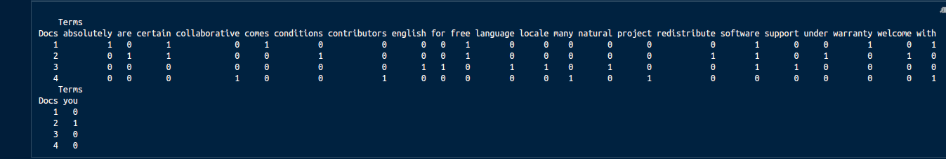
Let's say our document is "Free software comes with ABSOLUTELY NO certain WARRANTY","You are welcome to redistribute free software under certain conditions","Natural language support for software in an English locale","A collaborative project with many contributors".
The image below shows the matrix format of this document where every column represents a term from the document.
 Text Cleaning - It involves cleaning the text in following ways:
Remove words - If the data is extracted using web scraping, you might want to remove html tags.
Remove stop words - Stop words are a set of words which helps in sentence construction and don't have any real information.
Words such as a, an, the, they, where etc. are categorized as stop words.
Convert to lower - To maintain a standarization across all text and get rid of case differences and convert the entire text to lower.
Remove punctuation - We remove punctuation since they don't deliver any information.
Remove number - Similarly, we remove numerical figures from text
Remove whitespaces - Then, we remove the used spaces in the text.
Stemming & Lemmatization - Finally, we convert the terms into their root form.
For example: Words like playing, played, plays gets converted to the root word 'play'.
It helps in capturing the intent of terms precisely.
Feature Engineering - To be explained in the following section
Model Building - After the raw data is passed through all the above steps, it become ready for model building.
As mentioned above, not all ML algorithms perform well on text data.
Naive Bayes is popularly known to deliver high accuracy on text data.
In addition, deep neural network models also perform fairly well.
Text Cleaning - It involves cleaning the text in following ways:
Remove words - If the data is extracted using web scraping, you might want to remove html tags.
Remove stop words - Stop words are a set of words which helps in sentence construction and don't have any real information.
Words such as a, an, the, they, where etc. are categorized as stop words.
Convert to lower - To maintain a standarization across all text and get rid of case differences and convert the entire text to lower.
Remove punctuation - We remove punctuation since they don't deliver any information.
Remove number - Similarly, we remove numerical figures from text
Remove whitespaces - Then, we remove the used spaces in the text.
Stemming & Lemmatization - Finally, we convert the terms into their root form.
For example: Words like playing, played, plays gets converted to the root word 'play'.
It helps in capturing the intent of terms precisely.
Feature Engineering - To be explained in the following section
Model Building - After the raw data is passed through all the above steps, it become ready for model building.
As mentioned above, not all ML algorithms perform well on text data.
Naive Bayes is popularly known to deliver high accuracy on text data.
In addition, deep neural network models also perform fairly well.
What are Feature Engineering Techniques used in Text Mining ?
Do you know each word of this line you are reading can be converted into a feature ? Yes, you heard correctly.
Text data offers a wide range of possibilities to generate new features.
But sometimes, we end up generating lots of features, to an extent that processing them becomes a painful task.
Hence we should meticulously analyze the extracted features.
Don't worry! The methods explained below will also help in reducing the dimension of the resultant data set.
Below is the list of popular feature engineering methods used:
1. n-grams : In the document corpus, 1 word (such as baby, play, drink) is known as 1-gram.
Similarly, we can have 2-gram (baby toy, play station, diamond ring), 3-gram etc.
The idea behind this technique is to explore the chances that when one or two or more words occurs together gives more information to the model.
2. TF - IDF : It is also known as Term Frequency - Inverse Document Frequency.
This technique believes that, from a document corpus, a learning algorithm gets more information from the rarely occurring terms than frequently occurring terms.
Using a weighted scheme, this technique helps to score the importance of terms.
The terms occurring frequently are weighted lower and the terms occurring rarely get weighted higher.
* TF is be calculated as: frequency of a term in a document / all the terms in the document.
* IDF is calculated as: ratio of log (total documents in the corpus / number of documents with the 'term' in the corpus)
* Finally, TF-IDF is calculated as: TF X IDF.
Fortunately, R has packages which can do these calculations effort
3. Cosine Similarity - This measure helps to find similar documents.
It's one of the commonly used distance metric used in text analysis.
For a given 2 vectors A and B of length n each, cosine similarity can be calculated as a dot product of two unit vectors:
 4. Jaccard Similarity - This is another distance metric used in text analysis.
For a given two vectors (A and B), it can be calculated as ratio of (terms which are available in both vectors / terms which are available in either of the vectors).
It's formula is: (A ∩ B)/(A U B).
To create features using distance metrics, first we'll create cluster of similar documents and assign a unique label to each document in a new column.
5. Levenshtein Distance - We can also use levenshtein distance to create a new feature based on distance between two strings.
We won't go into its complicated formula, but understand what it does: it finds the shorter string in longer texts and returns the maximum value as 1 if both the shorter string is found.
For example: Calculating levenshtein distance for string "Alps Street 41" and "1st Block, Alps Street 41" will result in 1.
6. Feature Hashing - This technique implements the 'hashing trick' which helps in reducing the dimension of document matrix (lesser columns).
It doesn't use the actual data, instead it uses the indexes[i,j] of the data, thus it processes data only when needed.
And, that's why it takes lesser memory in computation.
In addition, there are more techniques which we'll discover while modeling text data in the next section.
4. Jaccard Similarity - This is another distance metric used in text analysis.
For a given two vectors (A and B), it can be calculated as ratio of (terms which are available in both vectors / terms which are available in either of the vectors).
It's formula is: (A ∩ B)/(A U B).
To create features using distance metrics, first we'll create cluster of similar documents and assign a unique label to each document in a new column.
5. Levenshtein Distance - We can also use levenshtein distance to create a new feature based on distance between two strings.
We won't go into its complicated formula, but understand what it does: it finds the shorter string in longer texts and returns the maximum value as 1 if both the shorter string is found.
For example: Calculating levenshtein distance for string "Alps Street 41" and "1st Block, Alps Street 41" will result in 1.
6. Feature Hashing - This technique implements the 'hashing trick' which helps in reducing the dimension of document matrix (lesser columns).
It doesn't use the actual data, instead it uses the indexes[i,j] of the data, thus it processes data only when needed.
And, that's why it takes lesser memory in computation.
In addition, there are more techniques which we'll discover while modeling text data in the next section.
Text Mining Practical - Predict the interest level
Since regular expressions help wonderfully in dealing with text data, make sure that you have referred to the regular expression tutorial as well.
Instead of a dummy data, we'll get our hands on a real text mining problem.
In this problem, we'll predict the popularity of apartment rental listing based on given features.
The data set has been taken from currently running two sigma rental listing problem on Kaggle.
Therefore, after you finish this tutorial, you can right away participate in it and try your luck.
Since the focus of this tutorial is text mining, we'll work only on the text features available in the data.
For this tutorial, you can download the data here. (huge dataset)
Now, we'll load the data and useful libraries for solving this problem.
Using map_at function from purrr package, we'll convert the json files into tabular data tables.
#load libraries
path <- "/home/manish/Desktop/Data2017/February/twosigma/"
setwd(path)
library(data.table)
library(jsonlite)
library(purrr) # big tool sets working with data wrangling.
library(RecordLinkage) # functions for data comparison and matching
library(stringr) # functions to make working with strings
library(tm) # for text mining applications
#load data
traind <- fromJSON("train.json")
test <- fromJSON("test.json")
#convert json to data table
vars <- setdiff(names(traind),c("photos","features"))
train <- map_at(traind, vars, unlist) %>% as.data.table() # Apply a function to each element of a vector conditionally
test <- map_at(test,vars,unlist) %>% as.data.table()
Since we are interested only in text variables, let's extract the text features:
train <- train[,.(listing_id,features, description,street_address,display_address,interest_level)]
test <- test[,.(listing_id,features,street_address,display_address,description)]
Let's quickly understand what the data is about:
we can derive the following insights:
dim(train) #The train data has 49352 rows and 6 columns.
dim(test) #The test data has 74659 rows and 5 columns.
head(train)
head(test)
sapply(train,class)
sapply(test,class)
interest_level is the dependent variable i.e. the variable to predict
listing_id variable has unique value for every listing.
In other words, it is the identifier variable.
features comprises of a list of features for every listing_id
description refers to the description of a listing_id provided by the agent
Street address and display address refers to the address of the listed apartment.
Let's start with the analysis.
We'll now join the data and create some new features.
#join data
test[,interest_level := "None"]
tdata <- rbindlist(list(train,test))
#fill empty values in the list
tdata[,features := ifelse(map(features, is_empty),"aempty",features)]
#count number of features per listing
tdata[,feature_count := unlist(lapply(features, length))]
#count number of words in description
tdata[,desc_word_count := str_count(description,pattern = "\\w+")]
#count total length of description
tdata[,desc_len := str_count(description)]
#similarity between address
tdata[,lev_sim := levenshteinDist(street_address,display_address)]
Feature engineering doesn't play by a fixed set of rules.
With a different data set, you'll always discover new potential set of features.
The best way to become at expert at feature engineering is solve different types of problems.
Anyhow, for this problem I've created the following variables:
Count of number of features per listing
Count of number of words in the description
Count of total length of the description
Similarity between street and display address using levenshtein distance
dim(tdata)
Now, the data has 10 variables and 680961 observations.
If you think these variables are too less for a machine learning algorithm to work best, hold tight.
In a while, our data dimension is going to explode.
We'll create more new features from the variable 'Features' and 'Description'.
Let's take them up one by one.
First, we'll transform the list 'Features' into one feature per row format.
#extract variables from features
fdata <- data.table(listing_id = rep(unlist(tdata$listing_id), lapply(tdata$features, length)), features = unlist(tdata$features))
head(fdata)
#convert features to lower
fdata[,features := unlist(lapply(features, tolower))]
Since not all the features will be useful, let's calculate the count of features and remove features which are occurring less than 100 times in the data.
#calculate count for every feature
fdata[,count := .N, features]
fdata[order(count)][1:20]
#keep features which occur 100 or more times
fdata <- fdata[count >= 100]
Let's convert each feature into a separate column so that it can be used as a variable in model training.
To accomplish that, we'll use the dcast function.
#convert columns into table
fdata <- dcast(data = fdata, formula = listing_id ~ features, fun.aggregate = length, value.var = "features")
dim(fdata)
This has resulted in 96 new variables.
We'll keep this new data set as is, and extract more features from the description variable.
From here, we'll be using tm package.
#create a corpus of descriptions
text_corpus <- Corpus(VectorSource(tdata$description))
#check first 4 documents
inspect(text_corpus[1:4])
#the corpus is a list object in R of type CORPUS
print(lapply(text_corpus[1:2], as.character))
As you can see, the word 'br' is just a noise and doesn't provide any useful information in the description.
We'll remove it.
Also, we'll perform the text mining steps to clean the data as explained in section above.
#let's clean the data
dropword <- "br"
#remove br
text_corpus <- tm_map(text_corpus,removeWords,dropword)
print(as.character(text_corpus[[1]]))
#tolower
text_corpus <- tm_map(text_corpus, tolower)
print(as.character(text_corpus[[1]]))
#remove punctuation
text_corpus <- tm_map(text_corpus, removePunctuation)
print(as.character(text_corpus[[1]]))
#remove number
text_corpus <- tm_map(text_corpus, removeNumbers)
print(as.character(text_corpus[[1]]))
#remove whitespaces
text_corpus <- tm_map(text_corpus, stripWhitespace,lazy = T)
print(as.character(text_corpus[[1]]))
#remove stopwords
text_corpus <- tm_map(text_corpus, removeWords, c(stopwords('english')))
print(as.character(text_corpus[[1]]))
#convert to text document
text_corpus <- tm_map(text_corpus, PlainTextDocument)
#perform stemming - this should always be performed after text doc conversion
text_corpus <- tm_map(text_corpus, stemDocument,language = "english")
print(as.character(text_corpus[[1]]))
text_corpus[[1]]$content
After every cleaning step, we've printed the resultant corpus to help you understand the effect of each step on the corpus.
Now, our corpus is ready to get converted into a matrix.
#convert to document term matrix
docterm_corpus <- DocumentTermMatrix(text_corpus)
dim(docterm_corpus)
This matrix has resulted in 52647 features.
Such matrices resulted from text data creates sparse matrices.
'Sparse' means most of the rows have zeroes.
In our matrix also, there could be columns which have > 90% zeroes or we can say, those columns are > 90% sparse.
Also, training models on such ultra high data dimensional data would take weeks to process.
Therefore, we'll remove the sparse terms.
Let's remove the variables which are 95% or more sparse.
new_docterm_corpus <- removeSparseTerms(docterm_corpus,sparse = 0.95)
dim(new_docterm_corpus)
Now, our matrix looks more friendly with 87 features.
But, which are these features ? It's equally important to explore and visualize the features to gain better understanding of the matrix.
Let's calculate the most frequent and least frequently occurring set of features.
#find frequent terms
colS <- colSums(as.matrix(new_docterm_corpus))
length(colS)
doc_features <- data.table(name = attributes(colS)$names, count = colS)
#most frequent and least frequent words
doc_features[order(-count)][1:10] #top 10 most frequent words
doc_features[order(count)][1:10] #least 10 frequent words
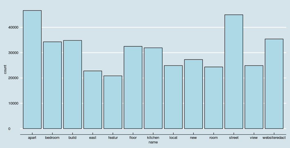
We can also visualize this table using simple bar plots.
To avoid overly populated bar chart, let's plot features occurring more than 20,000 times.
library(ggplot2)
library(ggthemes)
ggplot(doc_features[count>20000],aes(name, count)) + geom_bar(stat = "identity",fill='lightblue',color='black')+ theme(axis.text.x = element_text(angle = 45, hjust = 1))+ theme_economist()+ scale_color_economist()
#check association of terms of top features
findAssocs(new_docterm_corpus,"street",corlimit = 0.5)
findAssocs(new_docterm_corpus,"new",corlimit = 0.5)
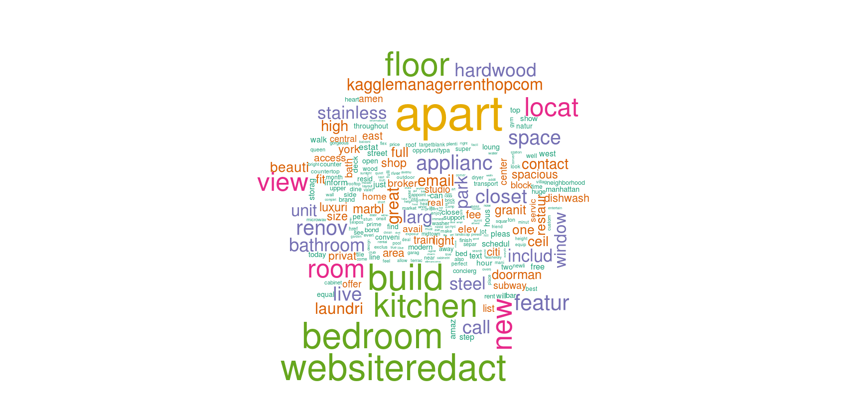
A better way to visualize text features is using a wordcloud.
A wordcloud is composed of words where the size of each word is determined by its frequency in the data.
In R, we'll use wordcloud package to do this task.
Let's create two word clouds with different frequencies.
#create wordcloud
library(wordcloud)
wordcloud(names(colS), colS, min.freq = 100, scale = c(6,.1), colors = brewer.pal(6, 'Dark2'))
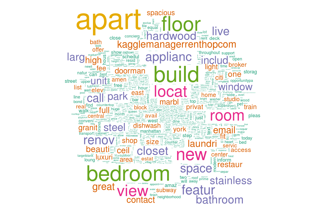
wordcloud(names(colS), colS, min.freq = 5000, scale = c(6,.1), colors = brewer.pal(6, 'Dark2'))
 Until here, we've chopped the description variable and extracted 87 features out of it.
The final step is to convert the matrix into a data frame and merge it with new features from 'Feature' column.
Until here, we've chopped the description variable and extracted 87 features out of it.
The final step is to convert the matrix into a data frame and merge it with new features from 'Feature' column.
#create data set for training
processed_data <- as.data.table(as.matrix(new_docterm_corpus))
#combing the data
data_one <- cbind(data.table(listing_id = tdata$listing_id, interest_level = tdata$interest_level),processed_data)
#merging the features
data_one <- fdata[data_one, on="listing_id"]
#split the data set into train and test
train_one <- data_one[interest_level != "None"]
test_one <- data_one[interest_level == "None"]
test_one[,interest_level := NULL]
Our data set is ready for training.
We'll use xgboost algorithm for model training.
If you are new to xgboost, I suggest you to refer this beginners tutorial on xgboost.
At core, xgboost learns from data using boosting algorithms where progressive models are build by capitalizing on errors made by previous models.
Xgboost follows a certain way of dealing with data:
It accepts dependent variable in integer format.
The data should be in matrix format
To check model performance, we can specify a validation set such that we can check validation errors during model training.
It is enable with both k-fold and hold-out validation strategy.
For faster training, we'll use hold-out validation strategy.
The training data must not have dependent variable.
It should be removed.
Neither, it should have the identifier variable (listing_id)
Keeping its nature in mind, let's prepare the data for xgboost and train our model.
library(caTools)
library(xgboost)
#stratified splitting the data
sp <- sample.split(Y = train_one$interest_level,SplitRatio = 0.6)
#create data for xgboost
xg_val <- train_one[sp]
listing_id <- train_one$listing_id
target <- train_one$interest_level
xg_val_target <- target[sp]
d_train <- xgb.DMatrix(data = as.matrix(train_one[,-c("listing_id","interest_level"),with=F]),label = target)
d_val <- xgb.DMatrix(data = as.matrix(xg_val[,-c("listing_id","interest_level"),with=F]), label = xg_val_target)
d_test <- xgb.DMatrix(data = as.matrix(test_one[,-c("listing_id"),with=F]))
param <- list(booster="gbtree", objective="multi:softprob", eval_metric="mlogloss", #nthread=13, num_class=3, eta = .02, gamma = 1, max_depth = 4, min_child_weight = 1, subsample = .7, colsample_bytree = .5 )
set.seed(2017)
watch <- list(val=d_val, train=d_train)
xgb2 <- xgb.train(data = d_train, params = param, watchlist=watch, nrounds = 500, print_every_n = 10 )
This model returns validation error = 0.6817.
The score is calculated with multilogloss metric.
Think of validation error as a proxy performance of model on future data.
Now, let's create predictions on test data and check our score on kaggle leaderboard.
xg_pred <- as.data.table(t(matrix(predict(xgb2, d_test), nrow=3, ncol=nrow(d_test))))
colnames(xg_pred) <- c("high","low","medium")
xg_pred <- cbind(data.table(listing_id = test$listing_id),xg_pred)
fwrite(xg_pred, "xgb_textmining.csv")
It gives us 0.7043 multilogloss score on leaderboard.
Not bad! We've used only 2 variables (features, description) from the data.
So, what can be done for improvement ? Obviously, we can pick up non-text variables from the original data and include them in model building.
Besides that, let's try few more text mining techniques.
What about TF-IDF matrix ? Here's an exercise for you.
We created processed_data as a data table from new_docterm_corpus.
It contained simple 1 and 0 to detect the presence of a new word in the description.
Let's create a weighted matrix using tf-idf technique.
It's quite easy to do.
#TF IDF Data set
data_mining_tf <- as.data.table(as.matrix(weightTfIdf(new_docterm_corpus)))
Here's your exercise one: Follow the steps above and calculate validation and leaderboard score on this data.
Does your score improve ? What else can be done ? Think! What about n - gram technique ? Until now, our matrix has one gram features i.e.
one word per column such as apart, new, building etc.
Now, we'll create a 2-gram document matrix and check model performance on it.
To create a n-gram matrix, we'll use NGramTokenizer function from Rweka package.
install.packages("RWeka")
library(RWeka)
#bigram function
Bigram_Tokenizer <- function(x){ NGramTokenizer(x, Weka_control(min=2, max=2)) }
#create a matrix
bi_docterm_matrix <- DocumentTermMatrix(text_corpus, control = list(tokenize = Bigram_Tokenizer))
Here's your exercise two: Create a data table from this bi_docterm_matrix and check your score.
Your next steps would are similar to what we've done above.
For your reference, following are the steps you should take:
Remove sparse terms
Explore the new features using bar chart and wordcloud
Convert the matrix into data table
Divide the resultant data table into train and test
Train and Test the models
Once this is done, check the leaderboard score.
Do let me know in comments if it got improved.
The complete script of this tutorial can be found here.
Summary
This tutorial is meant for beginners to get started with building text mining models.
Considering the massive volume of content being generated by companies, social media these days, there is going to be a surge in demand for people who are well versed with text mining & natural language processing.
This tutorial illustrates all the necessary steps which one must take while dealing with text data.
For better understanding, I would suggest you to get your hands on variety of text data sets and use the steps above for analysis.
Regardless of any programming language you use, these techniques & steps are common in all.
Did you find this tutorial helpful ? Feel free to drop your suggestions, doubts in the comments below.
Text Mining and Sentiment Analysis: Analysis with R
In the third article of this series, Sanil Mhatre demonstrates how to perform a sentiment analysis using R including generating a word cloud, word associations, sentiment scores, and emotion classification.
The series so far:
Introduction
Power BI Visualizations
Analysis with R
Oracle Text
Data Visualization in Tableau
Sentiment Analysis with Python
This is the third article of the “Text Mining and Sentiment Analysis” Series.
The first article introduced Azure Cognitive Services and demonstrated the setup and use of Text Analytics APIs for extracting key Phrases & Sentiment Scores from text data.
The second article demonstrated Power BI visualizations for analyzing Key Phrases & Sentiment Scores and interpreting them to gain insights.
This article explores R for text mining and sentiment analysis.
I will demonstrate several common text analytics techniques and visualizations in R.
Note: This article assumes basic familiarity with R and RStudio.
Please jump to the References section for more information on installing R and RStudio.
The Demo data raw text file and R script are available for download from my GitHub repository; please find the link in the References section.
R is a language and environment for statistical computing and graphics.
It provides a wide variety of statistical and graphical techniques and is highly extensible.
R is available as free software.
It’s easy to learn
and use and can produce well designed publication-quality plots.
For the demos in this article, I am using R version 3.5.3 (2019-03-11), RStudio Version 1.1.456
The input file for this article has only one column, the “Raw text” of survey responses and is a text file.
A sample of the first few rows are shown in Notepad++ (showing all characters) in Figure 1.
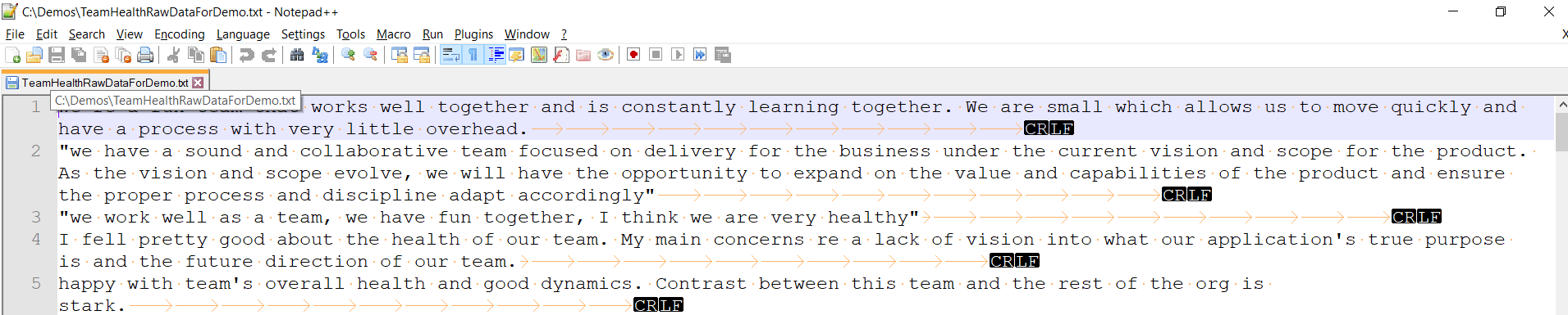 Figure 1. Sample of the input text file
The demo R script and demo input text file are available on my GitHub repo (please find the link in the References section).
R has a rich set of packages for Natural Language Processing (NLP) and generating plots.
The foundational steps involve loading the text file into an R Corpus, then cleaning and stemming the data before performing analysis.
I will demonstrate these steps and analysis like Word Frequency, Word Cloud, Word Association, Sentiment Scores and Emotion Classification using various plots and charts.
Installing and loading R packages
The following packages are used in the examples in this article:
tm for text mining operations like removing numbers, special characters, punctuations and stop words (Stop words in any language are the most commonly occurring words that have very little value for NLP and should be filtered out.
Examples of stop words in English are “the”, “is”, “are”.)
snowballc for stemming, which is the process of reducing words to their base or root form.
For example, a stemming algorithm would reduce the words “fishing”, “fished” and “fisher” to the stem “fish”.
wordcloud for generating the word cloud plot.
RColorBrewer for color palettes used in various plots
syuzhet for sentiment scores and emotion classification
ggplot2 for plotting graphs
Open RStudio and create a new R Script.
Use the following code to install and load these packages.
# Install
install.packages("tm") # for text mining
install.packages("SnowballC") # for text stemming
install.packages("wordcloud") # word-cloud generator
install.packages("RColorBrewer") # color palettes
install.packages("syuzhet") # for sentiment analysis
install.packages("ggplot2") # for plotting graphs
# Load
library("tm")
library("SnowballC")
library("wordcloud")
library("RColorBrewer")
library("syuzhet")
library("ggplot2")
Reading file data into R
The R base function
Figure 1. Sample of the input text file
The demo R script and demo input text file are available on my GitHub repo (please find the link in the References section).
R has a rich set of packages for Natural Language Processing (NLP) and generating plots.
The foundational steps involve loading the text file into an R Corpus, then cleaning and stemming the data before performing analysis.
I will demonstrate these steps and analysis like Word Frequency, Word Cloud, Word Association, Sentiment Scores and Emotion Classification using various plots and charts.
Installing and loading R packages
The following packages are used in the examples in this article:
tm for text mining operations like removing numbers, special characters, punctuations and stop words (Stop words in any language are the most commonly occurring words that have very little value for NLP and should be filtered out.
Examples of stop words in English are “the”, “is”, “are”.)
snowballc for stemming, which is the process of reducing words to their base or root form.
For example, a stemming algorithm would reduce the words “fishing”, “fished” and “fisher” to the stem “fish”.
wordcloud for generating the word cloud plot.
RColorBrewer for color palettes used in various plots
syuzhet for sentiment scores and emotion classification
ggplot2 for plotting graphs
Open RStudio and create a new R Script.
Use the following code to install and load these packages.
# Install
install.packages("tm") # for text mining
install.packages("SnowballC") # for text stemming
install.packages("wordcloud") # word-cloud generator
install.packages("RColorBrewer") # color palettes
install.packages("syuzhet") # for sentiment analysis
install.packages("ggplot2") # for plotting graphs
# Load
library("tm")
library("SnowballC")
library("wordcloud")
library("RColorBrewer")
library("syuzhet")
library("ggplot2")
Reading file data into R
The R base function read.table() is generally used to read a file in table format and imports data as a data frame.
Several variants of this function are available, for importing different file formats;
read.csv() is used for reading comma-separated value (csv) files, where a comma “,” is used a field separator
read.delim() is used for reading tab-separated values (.txt) files
The input file has multiple lines of text and no columns/fields (data is not tabular), so you will use the readLines function.
This function takes a file (or URL) as input and returns a vector containing as many elements as the number of lines in the file.
The readLines function simply extracts the text from its input source and returns each line as a character string.
The n= argument is useful to read a limited number (subset) of lines from the input source (Its default value is -1, which reads all lines from the input source).
When using the filename in this function’s argument, R assumes the file is in your current working directory (you can use the getwd() function in R console to find your current working directory).
You can also choose the input file interactively, using the file.choose() function within the argument.
The next step is to load that Vector as a Corpus.
In R, a Corpus is a collection of text document(s) to apply text mining or NLP routines on.
Details of using the readLines function are sourced from: https://www.stat.berkeley.edu/~spector/s133/Read.html .
In your R script, add the following code to load the data into a corpus.
# Read the text file from local machine , choose file interactively
text <- readLines(file.choose())
# Load the data as a corpus
TextDoc <- Corpus(VectorSource(text))
Upon running this, you will be prompted to select the input file.
Navigate to your file and click Open as shown in Figure 2.
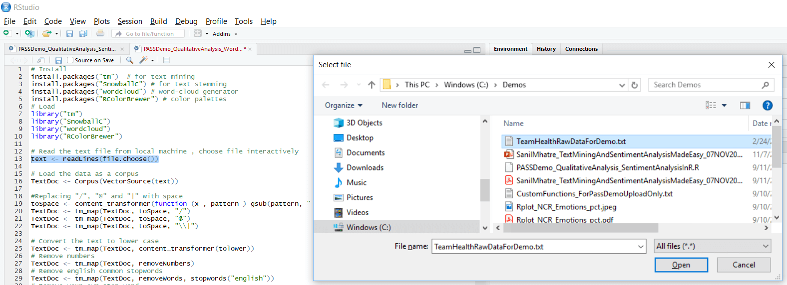 Figure 2.
Select input file
Cleaning up Text Data
Cleaning the text data starts with making transformations like removing special characters from the text.
This is done using the
Figure 2.
Select input file
Cleaning up Text Data
Cleaning the text data starts with making transformations like removing special characters from the text.
This is done using the tm_map() function to replace special characters like /, @ and | with a space.
The next step is to remove the unnecessary whitespace and convert the text to lower case.
Then remove the stopwords.
They are the most commonly occurring words in a language and have very little value in terms of gaining useful information.
They should be removed before performing further analysis.
Examples of stopwords in English are “the, is, at, on”.
There is no single universal list of stop words used by all NLP tools.
stopwords in the tm_map() function supports several languages like English, French, German, Italian, and Spanish.
Please note the language names are case sensitive.
I will also demonstrate how to add your own list of stopwords, which is useful in this Team Health example for removing non-default stop words like “team”, “company”, “health”.
Next, remove numbers and punctuation.
The last step is text stemming.
It is the process of reducing the word to its root form.
The stemming process simplifies the word to its common origin.
For example, the stemming process reduces the words “fishing”, “fished” and “fisher” to its stem “fish”.
Please note stemming uses the SnowballC package.
(You may want to skip the text stemming step if your users indicate a preference to see the original “unstemmed” words in the word cloud plot)
In your R script, add the following code to transform and run to clean-up the text data.
#Replacing "/", "@" and "|" with space
toSpace <- content_transformer(function (x , pattern ) gsub(pattern, " ", x))
TextDoc <- tm_map(TextDoc, toSpace, "/")
TextDoc <- tm_map(TextDoc, toSpace, "@")
TextDoc <- tm_map(TextDoc, toSpace, "\\|")
# Convert the text to lower case
TextDoc <- tm_map(TextDoc, content_transformer(tolower))
# Remove numbers
TextDoc <- tm_map(TextDoc, removeNumbers)
# Remove english common stopwords
TextDoc <- tm_map(TextDoc, removeWords, stopwords("english"))
# Remove your own stop word
# specify your custom stopwords as a character vector
TextDoc <- tm_map(TextDoc, removeWords, c("s", "company", "team"))
# Remove punctuations
TextDoc <- tm_map(TextDoc, removePunctuation)
# Eliminate extra white spaces
TextDoc <- tm_map(TextDoc, stripWhitespace)
# Text stemming - which reduces words to their root form
TextDoc <- tm_map(TextDoc, stemDocument)
Building the term document matrix
After cleaning the text data, the next step is to count the occurrence of each word, to identify popular or trending topics.
Using the function TermDocumentMatrix() from the text mining package, you can build a Document Matrix – a table containing the frequency of words.
In your R script, add the following code and run it to see the top 5 most frequently found words in your text.
# Build a term-document matrix
TextDoc_dtm <- TermDocumentMatrix(TextDoc)
dtm_m <- as.matrix(TextDoc_dtm)
# Sort by descearing value of frequency
dtm_v <- sort(rowSums(dtm_m),decreasing=TRUE)
dtm_d <- data.frame(word = names(dtm_v),freq=dtm_v)
# Display the top 5 most frequent words
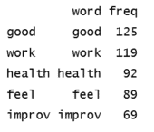
head(dtm_d, 5)
The following table of word frequency is the expected output of the head command on RStudio Console.
 Plotting the top 5 most frequent words using a bar chart is a good basic way to visualize this word frequent data.
In your R script, add the following code and run it to generate a bar chart, which will display in the Plots sections of RStudio.
# Plot the most frequent words
barplot(dtm_d[1:5,]$freq, las = 2, names.arg = dtm_d[1:5,]$word,
col ="lightgreen", main ="Top 5 most frequent words",
ylab = "Word frequencies")
The plot can be seen in Figure 3.
Plotting the top 5 most frequent words using a bar chart is a good basic way to visualize this word frequent data.
In your R script, add the following code and run it to generate a bar chart, which will display in the Plots sections of RStudio.
# Plot the most frequent words
barplot(dtm_d[1:5,]$freq, las = 2, names.arg = dtm_d[1:5,]$word,
col ="lightgreen", main ="Top 5 most frequent words",
ylab = "Word frequencies")
The plot can be seen in Figure 3.
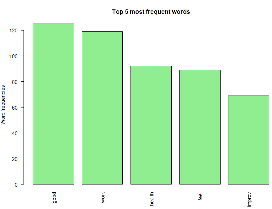 Figure 3.
Bar chart of the top 5 most frequent words
One could interpret the following from this bar chart:
The most frequently occurring word is “good”.
Also notice that negative words like “not” don’t feature in the bar chart, which indicates there are no negative prefixes to change the context or meaning of the word “good” ( In short, this indicates most responses don’t mention negative phrases like “not good”).
“work”, “health” and “feel” are the next three most frequently occurring words, which indicate that most people feel good about their work and their team’s health.
Finally, the root “improv” for words like “improve”, “improvement”, “improving”, etc.
is also on the chart, and you need further analysis to infer if its context is positive or negative
Generate the Word Cloud
A word cloud is one of the most popular ways to visualize and analyze qualitative data.
It’s an image composed of keywords found within a body of text, where the size of each word indicates its frequency in that body of text.
Use the word frequency data frame (table) created previously to generate the word cloud.
In your R script, add the following code and run it to generate the word cloud and display it in the Plots section of RStudio.
#generate word cloud
set.seed(1234)
wordcloud(words = dtm_d$word, freq = dtm_d$freq, min.freq = 5,
max.words=100, random.order=FALSE, rot.per=0.40,
colors=brewer.pal(8, "Dark2"))
Below is a brief description of the arguments used in the word cloud function;
words – words to be plotted
freq – frequencies of words
min.freq – words whose frequency is at or above this threshold value is plotted (in this case, I have set it to 5)
max.words – the maximum number of words to display on the plot (in the code above, I have set it 100)
random.order – I have set it to FALSE, so the words are plotted in order of decreasing frequency
rot.per – the percentage of words that are displayed as vertical text (with 90-degree rotation).
I have set it 0.40 (40 %), please feel free to adjust this setting to suit your preferences
colors – changes word colors going from lowest to highest frequencies
You can see the resulting word cloud in Figure 4.
Figure 3.
Bar chart of the top 5 most frequent words
One could interpret the following from this bar chart:
The most frequently occurring word is “good”.
Also notice that negative words like “not” don’t feature in the bar chart, which indicates there are no negative prefixes to change the context or meaning of the word “good” ( In short, this indicates most responses don’t mention negative phrases like “not good”).
“work”, “health” and “feel” are the next three most frequently occurring words, which indicate that most people feel good about their work and their team’s health.
Finally, the root “improv” for words like “improve”, “improvement”, “improving”, etc.
is also on the chart, and you need further analysis to infer if its context is positive or negative
Generate the Word Cloud
A word cloud is one of the most popular ways to visualize and analyze qualitative data.
It’s an image composed of keywords found within a body of text, where the size of each word indicates its frequency in that body of text.
Use the word frequency data frame (table) created previously to generate the word cloud.
In your R script, add the following code and run it to generate the word cloud and display it in the Plots section of RStudio.
#generate word cloud
set.seed(1234)
wordcloud(words = dtm_d$word, freq = dtm_d$freq, min.freq = 5,
max.words=100, random.order=FALSE, rot.per=0.40,
colors=brewer.pal(8, "Dark2"))
Below is a brief description of the arguments used in the word cloud function;
words – words to be plotted
freq – frequencies of words
min.freq – words whose frequency is at or above this threshold value is plotted (in this case, I have set it to 5)
max.words – the maximum number of words to display on the plot (in the code above, I have set it 100)
random.order – I have set it to FALSE, so the words are plotted in order of decreasing frequency
rot.per – the percentage of words that are displayed as vertical text (with 90-degree rotation).
I have set it 0.40 (40 %), please feel free to adjust this setting to suit your preferences
colors – changes word colors going from lowest to highest frequencies
You can see the resulting word cloud in Figure 4.
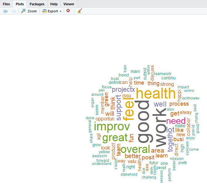 Figure 4.
Word cloud plot
The word cloud shows additional words that occur frequently and could be of interest for further analysis.
Words like “need”, “support”, “issu” (root for “issue(s)”, etc.
could provide more context around the most frequently occurring words and help to gain a better understanding of the main themes.
Word Association
Correlation is a statistical technique that can demonstrate whether, and how strongly, pairs of variables are related.
This technique can be used effectively to analyze which words occur most often in association with the most frequently occurring words in the survey responses, which helps to see the context around these words
In your R script, add the following code and run it.
# Find associations
findAssocs(TextDoc_dtm, terms = c("good","work","health"), corlimit = 0.25)
You should see the results as shown in Figure 5.
Figure 4.
Word cloud plot
The word cloud shows additional words that occur frequently and could be of interest for further analysis.
Words like “need”, “support”, “issu” (root for “issue(s)”, etc.
could provide more context around the most frequently occurring words and help to gain a better understanding of the main themes.
Word Association
Correlation is a statistical technique that can demonstrate whether, and how strongly, pairs of variables are related.
This technique can be used effectively to analyze which words occur most often in association with the most frequently occurring words in the survey responses, which helps to see the context around these words
In your R script, add the following code and run it.
# Find associations
findAssocs(TextDoc_dtm, terms = c("good","work","health"), corlimit = 0.25)
You should see the results as shown in Figure 5.
![A screenshot of a cell phone
Description automatically generated]() Figure 5.
Word association analysis for the top three most frequent terms
This script shows which words are most frequently associated with the top three terms (
Figure 5.
Word association analysis for the top three most frequent terms
This script shows which words are most frequently associated with the top three terms (corlimit = 0.25 is the lower limit/threshold I have set.
You can set it lower to see more words, or higher to see less).
The output indicates that “integr” (which is the root for word “integrity”) and “synergi” (which is the root for words “synergy”, “synergies”, etc.) and occur 28% of the time with the word “good”.
You can interpret this as the context around the most frequently occurring word (“good”) is positive.
Similarly, the root of the word “together” is highly correlated with the word “work”.
This indicates that most responses are saying that teams “work together” and can be interpreted in a positive context.
You can modify the above script to find terms associated with words that occur at least 50 times or more, instead of having to hard code the terms in your script.
# Find associations for words that occur at least 50 times
findAssocs(TextDoc_dtm, terms = findFreqTerms(TextDoc_dtm, lowfreq = 50), corlimit = 0.25)
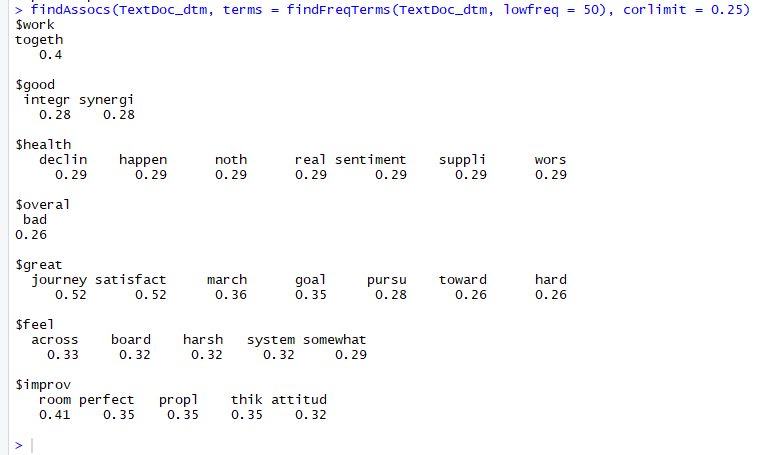 Figure 6: Word association output for terms occurring at least 50 times
Sentiment Scores
Sentiments can be classified as positive, neutral or negative.
They can also be represented on a numeric scale, to better express the degree of positive or negative strength of the sentiment contained in a body of text.
This example uses the Syuzhet package for generating sentiment scores, which has four sentiment dictionaries and offers a method for accessing the sentiment extraction tool developed in the NLP group at Stanford.
The
Figure 6: Word association output for terms occurring at least 50 times
Sentiment Scores
Sentiments can be classified as positive, neutral or negative.
They can also be represented on a numeric scale, to better express the degree of positive or negative strength of the sentiment contained in a body of text.
This example uses the Syuzhet package for generating sentiment scores, which has four sentiment dictionaries and offers a method for accessing the sentiment extraction tool developed in the NLP group at Stanford.
The get_sentiment function accepts two arguments: a character vector (of sentences or words) and a method.
The selected method determines which of the four available sentiment extraction methods will be used.
The four methods are syuzhet (this is the default), bing, afinn and nrc.
Each method uses a different scale and hence returns slightly different results.
Please note the outcome of nrc method is more than just a numeric score, requires additional interpretations and is out of scope for this article.
The descriptions of the get_sentiment function has been sourced from : https://cran.r-project.org/web/packages/syuzhet/vignettes/syuzhet-vignette.html?
Add the following code to the R script and run it.
# regular sentiment score using get_sentiment() function and method of your choice
# please note that different methods may have different scales
syuzhet_vector <- get_sentiment(text, method="syuzhet")
# see the first row of the vector
head(syuzhet_vector)
# see summary statistics of the vector
summary(syuzhet_vector)
Your results should look similar to Figure 7.
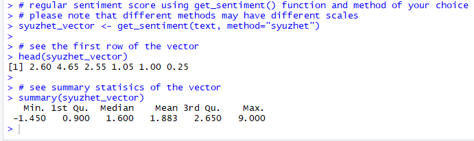 Figure 7. Syuzhet vector
An inspection of the Syuzhet vector shows the first element has the value of 2.60.
It means the sum of the sentiment scores of all meaningful words in the first response(line) in the text file, adds up to 2.60.
The scale for sentiment scores using the
Figure 7. Syuzhet vector
An inspection of the Syuzhet vector shows the first element has the value of 2.60.
It means the sum of the sentiment scores of all meaningful words in the first response(line) in the text file, adds up to 2.60.
The scale for sentiment scores using the syuzhet method is decimal and ranges from -1(indicating most negative) to +1(indicating most positive).
Note that the summary statistics of the suyzhet vector show a median value of 1.6, which is above zero and can be interpreted as the overall average sentiment across all the responses is positive.
Next, run the same analysis for the remaining two methods and inspect their respective vectors.
Add the following code to the R script and run it.
# bing
bing_vector <- get_sentiment(text, method="bing")
head(bing_vector)
summary(bing_vector)
#affin
afinn_vector <- get_sentiment(text, method="afinn")
head(afinn_vector)
summary(afinn_vector)
Your results should resemble Figure 8.
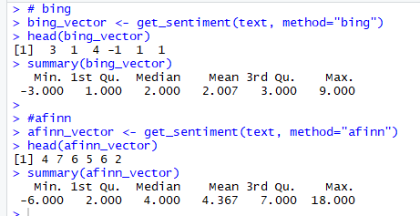 Figure 8. bing and afinn vectors
Please note the scale of sentiment scores generated by:
bing – binary scale with -1 indicating negative and +1 indicating positive sentiment
afinn – integer scale ranging from -5 to +5
The summary statistics of
Figure 8. bing and afinn vectors
Please note the scale of sentiment scores generated by:
bing – binary scale with -1 indicating negative and +1 indicating positive sentiment
afinn – integer scale ranging from -5 to +5
The summary statistics of bing and afinn vectors also show that the Median value of Sentiment scores is above 0 and can be interpreted as the overall average sentiment across the all the responses is positive.
Because these different methods use different scales, it’s better to convert their output to a common scale before comparing them.
This basic scale conversion can be done easily using R’s built-in sign function, which converts all positive number to 1, all negative numbers to -1 and all zeros remain 0.
Add the following code to your R script and run it.
#compare the first row of each vector using sign function
rbind(
sign(head(syuzhet_vector)),
sign(head(bing_vector)),
sign(head(afinn_vector))
)
Figure 9 shows the results.
![A screenshot of a cell phone
Description automatically generated]() Figure 9.
Normalize scale and compare three vectors
Note the first element of each row (vector) is 1, indicating that all three methods have calculated a positive sentiment score, for the first response (line) in the text.
Emotion Classification
Emotion classification is built on the NRC Word-Emotion Association Lexicon (aka EmoLex).
The definition of “NRC Emotion Lexicon”, sourced from http://saifmohammad.com/WebPages/NRC-Emotion-Lexicon.htm is “The NRC Emotion Lexicon is a list of English words and their associations with eight basic emotions (anger, fear, anticipation, trust, surprise, sadness, joy, and disgust) and two sentiments (negative and positive).
The annotations were manually done by crowdsourcing.”
To understand this, explore the
Figure 9.
Normalize scale and compare three vectors
Note the first element of each row (vector) is 1, indicating that all three methods have calculated a positive sentiment score, for the first response (line) in the text.
Emotion Classification
Emotion classification is built on the NRC Word-Emotion Association Lexicon (aka EmoLex).
The definition of “NRC Emotion Lexicon”, sourced from http://saifmohammad.com/WebPages/NRC-Emotion-Lexicon.htm is “The NRC Emotion Lexicon is a list of English words and their associations with eight basic emotions (anger, fear, anticipation, trust, surprise, sadness, joy, and disgust) and two sentiments (negative and positive).
The annotations were manually done by crowdsourcing.”
To understand this, explore the get_nrc_sentiments function, which returns a data frame with each row representing a sentence from the original file.
The data frame has ten columns (one column for each of the eight emotions, one column for positive sentiment valence and one for negative sentiment valence).
The data in the columns (anger, anticipation, disgust, fear, joy, sadness, surprise, trust, negative, positive) can be accessed individually or in sets.
The definition of get_nrc_sentiments has been sourced from: https://cran.r-project.org/web/packages/syuzhet/vignettes/syuzhet-vignette.html?
Add the following line to your R script and run it, to see the data frame generated from the previous execution of the get_nrc_sentiment function.
# run nrc sentiment analysis to return data frame with each row classified as one of the following
# emotions, rather than a score:
# anger, anticipation, disgust, fear, joy, sadness, surprise, trust
# It also counts the number of positive and negative emotions found in each row
d<-get_nrc_sentiment(text)
# head(d,10) - to see top 10 lines of the get_nrc_sentiment dataframe
head (d,10)
The results should look like Figure 10.
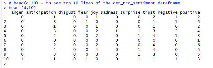 Figure 10. Data frame returned by get_nrc_sentiment function
The output shows that the first line of text has;
Zero occurrences of words associated with emotions of anger, disgust, fear, sadness and surprise
One occurrence each of words associated with emotions of anticipation and joy
Two occurrences of words associated with emotions of trust
Total of one occurrence of words associated with negative emotions
Total of two occurrences of words associated with positive emotions
The next step is to create two plots charts to help visually analyze the emotions in this survey text.
First, perform some data transformation and clean-up steps before plotting charts.
The first plot shows the total number of instances of words in the text, associated with each of the eight emotions.
Add the following code to your R script and run it.
#transpose
td<-data.frame(t(d))
#The function rowSums computes column sums across rows for each level of a grouping variable.
td_new <- data.frame(rowSums(td[2:253]))
#Transformation and cleaning
names(td_new)[1] <- "count"
td_new <- cbind("sentiment" = rownames(td_new), td_new)
rownames(td_new) <- NULL
td_new2<-td_new[1:8,]
#Plot One - count of words associated with each sentiment
quickplot(sentiment, data=td_new2, weight=count, geom="bar", fill=sentiment, ylab="count")+ggtitle("Survey sentiments")
You can see the bar plot in Figure 11.
Figure 10. Data frame returned by get_nrc_sentiment function
The output shows that the first line of text has;
Zero occurrences of words associated with emotions of anger, disgust, fear, sadness and surprise
One occurrence each of words associated with emotions of anticipation and joy
Two occurrences of words associated with emotions of trust
Total of one occurrence of words associated with negative emotions
Total of two occurrences of words associated with positive emotions
The next step is to create two plots charts to help visually analyze the emotions in this survey text.
First, perform some data transformation and clean-up steps before plotting charts.
The first plot shows the total number of instances of words in the text, associated with each of the eight emotions.
Add the following code to your R script and run it.
#transpose
td<-data.frame(t(d))
#The function rowSums computes column sums across rows for each level of a grouping variable.
td_new <- data.frame(rowSums(td[2:253]))
#Transformation and cleaning
names(td_new)[1] <- "count"
td_new <- cbind("sentiment" = rownames(td_new), td_new)
rownames(td_new) <- NULL
td_new2<-td_new[1:8,]
#Plot One - count of words associated with each sentiment
quickplot(sentiment, data=td_new2, weight=count, geom="bar", fill=sentiment, ylab="count")+ggtitle("Survey sentiments")
You can see the bar plot in Figure 11.
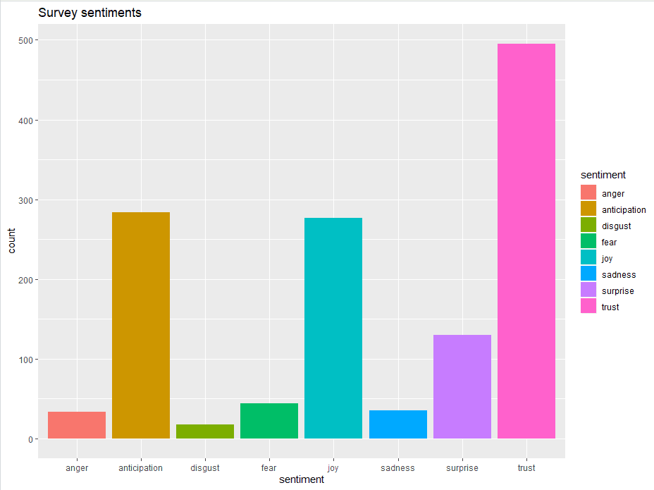 Figure 11. Bar Plot showing the count of words in the text, associated with each emotion
This bar chart demonstrates that words associated with the positive emotion of “trust” occurred about five hundred times in the text, whereas words associated with the negative emotion of “disgust” occurred less than 25 times.
A deeper understanding of the overall emotions occurring in the survey response can be gained by comparing these number as a percentage of the total number of meaningful words.
Add the following code to your R script and run it.
#Plot two - count of words associated with each sentiment, expressed as a percentage
barplot(
sort(colSums(prop.table(d[, 1:8]))),
horiz = TRUE,
cex.names = 0.7,
las = 1,
main = "Emotions in Text", xlab="Percentage"
)
The Emotions bar plot can be seen in figure 12.
Figure 11. Bar Plot showing the count of words in the text, associated with each emotion
This bar chart demonstrates that words associated with the positive emotion of “trust” occurred about five hundred times in the text, whereas words associated with the negative emotion of “disgust” occurred less than 25 times.
A deeper understanding of the overall emotions occurring in the survey response can be gained by comparing these number as a percentage of the total number of meaningful words.
Add the following code to your R script and run it.
#Plot two - count of words associated with each sentiment, expressed as a percentage
barplot(
sort(colSums(prop.table(d[, 1:8]))),
horiz = TRUE,
cex.names = 0.7,
las = 1,
main = "Emotions in Text", xlab="Percentage"
)
The Emotions bar plot can be seen in figure 12.
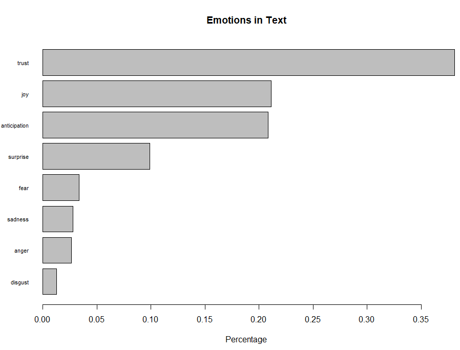 Figure 12. Bar Plot showing the count of words associated with each sentiment expressed as a percentage
This bar plot allows for a quick and easy comparison of the proportion of words associated with each emotion in the text.
The emotion “trust” has the longest bar and shows that words associated with this positive emotion constitute just over 35% of all the meaningful words in this text.
On the other hand, the emotion of “disgust” has the shortest bar and shows that words associated with this negative emotion constitute less than 2% of all the meaningful words in this text.
Overall, words associated with the positive emotions of “trust” and “joy” account for almost 60% of the meaningful words in the text, which can be interpreted as a good sign of team health.
Conclusion
This article demonstrated reading text data into R, data cleaning and transformations.
It demonstrated how to create a word frequency table and plot a word cloud, to identify prominent themes occurring in the text.
Word association analysis using correlation, helped gain context around the prominent themes.
It explored four methods to generate sentiment scores, which proved useful in assigning a numeric value to strength (of positivity or negativity) of sentiments in the text and allowed interpreting that the average sentiment through the text is trending positive.
Lastly, it demonstrated how to implement an emotion classification with NRC sentiment and created two plots to analyze and interpret emotions found in the text.
Figure 12. Bar Plot showing the count of words associated with each sentiment expressed as a percentage
This bar plot allows for a quick and easy comparison of the proportion of words associated with each emotion in the text.
The emotion “trust” has the longest bar and shows that words associated with this positive emotion constitute just over 35% of all the meaningful words in this text.
On the other hand, the emotion of “disgust” has the shortest bar and shows that words associated with this negative emotion constitute less than 2% of all the meaningful words in this text.
Overall, words associated with the positive emotions of “trust” and “joy” account for almost 60% of the meaningful words in the text, which can be interpreted as a good sign of team health.
Conclusion
This article demonstrated reading text data into R, data cleaning and transformations.
It demonstrated how to create a word frequency table and plot a word cloud, to identify prominent themes occurring in the text.
Word association analysis using correlation, helped gain context around the prominent themes.
It explored four methods to generate sentiment scores, which proved useful in assigning a numeric value to strength (of positivity or negativity) of sentiments in the text and allowed interpreting that the average sentiment through the text is trending positive.
Lastly, it demonstrated how to implement an emotion classification with NRC sentiment and created two plots to analyze and interpret emotions found in the text.
Basic Text Analysis
Character Encoding
One of the first things that is important to learn about quantitative text analysis is to most computer programs, texts or strings also have a numerical basis called character encoding.
Character encoding is a style of writing text in computer code that helps programs such as web browsers figure out how to display text.
There are presently dozens of different types of character encoding that resulted not only from advances in computing technology—and the development of different styles for different operating systems—but also for different languages (and even new languages such as emoji).
The figure below illustrates a form of character encoding called “Latin Extended-B” which was developed for representing text in languages derived from Latin (which of course excludes a number of important languages)
 Why should you care that text can be created using different forms of character encoding? Well, if you have scraped a large amount of data from multiple websites—or multiple social media sites— you may find that your data exist in multiple types of character encoding, and this can create a big hassle.
Before we begin working with a text-based dataset, it is useful to either a) make sure every text uses the same character encoding; or b) use a tool to force or coerce all text into a single character encoding.
The
Why should you care that text can be created using different forms of character encoding? Well, if you have scraped a large amount of data from multiple websites—or multiple social media sites— you may find that your data exist in multiple types of character encoding, and this can create a big hassle.
Before we begin working with a text-based dataset, it is useful to either a) make sure every text uses the same character encoding; or b) use a tool to force or coerce all text into a single character encoding.
The Encoding and inconv functions in base R can be very useful for the latter purposes.
Note, however, that the latter function may create “place holders” for characters that it cannot process.
For example, if an old version of character encoding is applied to text that contains emoji, the emoji may appear as strings of seeminly incoherent symbols and punctuation marks.
Inconsistent character encoding is one of the most common pitfalls for those attempting to learn how to perform quantitative text analysis in R, but there are no easy solutions.
If you try to run the code below and receive error messages such as invalid multibyte string, this is indicative of a character encoding issue that you will most likely need to resolve using one of the imperfect steps above.
GREP
Another important tool for working with text is GREP, which stands for “Globally search a regular expression and print.” In laymans terms, GREP is a tool that helps you search for the presence of a string of characters that matches a pattern.
To demonstrate why you need to learn some GREP, let’s return to an issue we encountered in a previous tutorial on screen-scraping.
In that tutorial, we scraped a Wikipedia page and discovered that there were strange characters such as \t and \n interspersed throughout the text we scraped.
At the time, I mentioned that these are html tags, or chunks of code that tell your web browser how to display something (in this case a “tab” space and a new line).
Let’s create a character string that includes such characters as follows (the meaning of the text isn’t important- this was scraped from the Duke University web page “Events” section):
wikipedia_scrape<- "Class of 2018: Senior Stories of Discovery, Learning and Serving\n\n\t\t\t\t\t\t\t"
Once again, GREP-style commands search for a certain pattern.
For example, let’s write some code that determines whether the word “Class” is part of our string using the grepl function in base R:
grepl("Class", wikipedia_scrape)
## [1] TRUE
The text within quotes is the pattern we are trying to find, and the second argument is the string we want to search within.
The output tells us that there was one occurrence of “Class.”
Now let’s use the gsub command to remove all \ts from the string
gsub("\t", ", wikipedia_scrape)
## [1] "Class of 2018: Senior Stories of Discovery, Learning and Serving\n\n"
The first argument in the gsub function names the pattern we are looking for, the second (blank) argument tells us what we want to replace that pattern with, and the third argument is the strong we want to transform.
We can also pass two arguments at once using the | separator as follows:
gsub("\t|\n", ", wikipedia_scrape)
## [1] "Class of 2018: Senior Stories of Discovery, Learning and Serving"
GREP-style commands also include a wildcard which can be used to, for example, find all words in a string that start with a certain letter, such as “P”:
some_text<-c("This","Professor","is","not","so","great")
some_text[grep("^[P]", some_text)]
## [1] "Professor"
Here is a useful cheatsheet that includes more examples of how to use GREP to find patterns in text.
Grep commands are fairly straight forward, and much more powerful and useful for subsetting rows or columns within larger datasets.
There is one more concept which is important for you to grasp about GREP, however, which is that certain characters such as " confuse the techniques.
For example
text_chunk<-c("[This Professor is not so Great]")
gsub("\",", text_chunk)
We receive an error message when we run the code above because the \ character has a literal meaning to R because it is part of something called a regular expression.
To remove this character, and other characters like it, we need to “escape” the character using single quotation marks wraped around a double \\ as follows:
text_chunk<-c("[This Professor is not so Great]")
gsub('\\[|\\]',", text_chunk)
## [1] "This Professor is not so Great"
Tokenization
Another important concept that is necessary to master to perform quantitative text analysis is Tokenization.
Tokenization refers to the way you are definining the unit of analysis.
This might include words, sequences of words, or entire sentences.
The figure below provides an example of one way to Tokenize a simple sentence.
 This figure illustrates the most common way of tokenizing a text—by individual word.
Many techniques in quantitative text analysis also analyze what are known as “n-grams” however.
Ngrams are simply sequences of words with length “n.” For example, the sentence above could be written in ngram form as “the quick brown”,“quick brown fox”, “brown fox jumps” and so on.
N-grams can be useful when word-order is important, as I will discuss in additional detail below.
For now, let me give you a simple example: “I hate the president” and “I’d hate to be the president.”
This figure illustrates the most common way of tokenizing a text—by individual word.
Many techniques in quantitative text analysis also analyze what are known as “n-grams” however.
Ngrams are simply sequences of words with length “n.” For example, the sentence above could be written in ngram form as “the quick brown”,“quick brown fox”, “brown fox jumps” and so on.
N-grams can be useful when word-order is important, as I will discuss in additional detail below.
For now, let me give you a simple example: “I hate the president” and “I’d hate to be the president.”
Creating a Corpus
Another unique feature of quantitative text analysis is that it typically requires new data formats that allow algorithms to quickly compare one document to a lot of other documents in order to identify patterns in word usage that can be used to identify latent themes, or address the overall popularity of a word or words in a single document vs.
a group of documents.
One of the most common data formats in the field of Natural Language Processing is a corpus.
In R, the tm package is often used to create a corpus object.
This package can be used to read in data in many different formats– including text within data frames, .txt files, or .doc files.
Let’s begin with an example of how to read in text from within a data frame.
We begin by loading an .Rdata file that contains 3,196 recent tweets by President Trump that are hosted on my Github page:
load(url("https://cbail.github.io/Trump_Tweets.Rdata"))
head(trumptweets$text)
## [1] "Just met with UN Secretary-General António Guterres who is working hard to “Make the United Nations Great Again.” When the UN does more to solve conflicts around the world, it means the U.S.
has less to do and we save money.
@NikkiHaley is doing a fantastic job! https://t.co/pqUv6cyH2z"
## [2] "America is a Nation that believes in the power of redemption.
America is a Nation that believes in second chances - and America is a Nation that believes that the best is always yet to come! #PrisonReform https://t.co/Yk5UJUYgHN"
## [3] "RT @SteveForbesCEO: .@realDonaldTrump speech on drug costs pays immediate dividends.
New @Amgen drug lists at 30% less than expected.
Middl…"
## [4] "We grieve for the terrible loss of life, and send our support and love to everyone affected by this horrible attack in Texas.
To the students, families, teachers and personnel at Santa Fe High School – we are with you in this tragic hour, and we will be with you forever...
https://t.co/LtJ0D29Hsv"
## [5] "School shooting in Texas.
Early reports not looking good.
God bless all!"
## [6] "Reports are there was indeed at least one FBI representative implanted, for political purposes, into my campaign for president.
It took place very early on, and long before the phony Russia Hoax became a “hot” Fake News story.
If true - all time biggest political scandal!"
In order to create a corpus of these tweets, we need to use the Corpus function within the tm package.
First let’s install that package
install.packages("tm")
Now let’s load the tm package in order to use its Corpus function:
library(tm)
## Loading required package: NLP
trump_corpus <- Corpus(VectorSource(as.vector(trumptweets$text)))
trump_corpus
## <<SimpleCorpus>>
## Metadata:  corpus specific: 1, document level (indexed): 0
## Content:  documents: 3196
As this output shows, we’ve created a corpus with 3,196 documents, where each document is one of Trump’s tweets.
You may also notice that the Corpus object can also store metadata such as information about the names of the author of each document of or the date each document was produced (though we are not storing any such meta data here.
Tidy-Text
An important alternative to Corpus object has emerged in recent years in the form of tidytext.
Instead of saving a group of documents and associated meta data, text that is in tidytext format contains one word per row, and each row also includes additional information about the name of the document where the word appears, and the order in which the words appear.
Let’s install the tidytext package to illustrate:
install.packages("tidytext")
Now let’s load our database of Trump tweets into tidytext format— since the tidytext package is part of the tidyverse, which is a family of packages that work well together in R that includes other popular packages such as dplyr and ggplot2 we will use the “piping” style of coding (%>%) associated with such packages:
library(tidytext)
library(dplyr)
tidy_trump_tweets<- trumptweets %>%
   select(created_at,text) %>%
   unnest_tokens("word", text)
A major advantage of tidytext format is that once the text has been tidy-ed, regular R functions can be used to analyze it instead of the specialized functions necessary to analyze a Corpus object.
For example, to count the most popular words in Trump’s tweets, we can do the following:
tidy_trump_tweets %>%
 count(word) %>%
   arrange(desc(n))
## # A tibble: 8,690 x 2
##    word      n
##    <chr> <int>
##  1 the    3671
##  2 to     2216
##  3 and    1959
##  4 of     1606
##  5 https  1281
##  6 t.co   1258
##  7 a      1248
##  8 in     1213
##  9 is     1045
## 10 for     886
## # ...
with 8,680 more rows
Not very informative or interesting that the most frequent word used by trump is “the” is it? This brings us to our next subject: text pre-processing.
Text Pre-Processing
Before we begin running quantitative analyses of text, we first need to decide precisely which type of text should be included in our analyses.
For example, as the code above showed, very common words such as “the” are often not very informative.
That is, we typically do not care if one author uses the word “the” more often than another in most forms of quantitative text analysis, but we might care a lot about how many times a politician uses the word “economy” on Twitter.
Stopwords
Common words such as “the”,“and”,“bot”,“for”,“is” etc.
are often described as “stop words,” meaning that they should not be included in a quantitative text analysis.
Removing stop words is fairly easy regardless of whether you are working with a Corpus object or a tidytext object assuming you are working with a widely used language such as English.
Let’s begin with the former, using the tm_map function as follows:
trump_corpus <- tm_map(trump_corpus, removeWords, stopwords("english"))
In tidytext we can remove stopwords as follows:
 data("stop_words")
   tidy_trump_tweets<-tidy_trump_tweets %>%
     anti_join(stop_words)
And now we can repeat the count of top words above:
tidy_trump_tweets %>%
 count(word) %>%
   arrange(desc(n))
## # A tibble: 8,121 x 2
##    word          n
##    <chr>     <int>
##  1 https      1281
##  2 t.co       1258
##  3 amp         562
##  4 rt          351
##  5 people      302
##  6 news        271
##  7 president   235
##  8 fake        234
##  9 trump       218
## 10 country     213
## # ...
with 8,111 more rows
Looks better, but we still have a number of terms in there that might not be very useful such as “https” or “t.co”, which is an abbreviation used in links shared on twitter.
Likewise “rt” is an abbreviation for “retweet,” and does not thus carry much meaning.
If we wanted to remove these words, we could create a custom list of stop words in the form of a character vector, and use the same anti_join function above to remove all words within this custom list.
Punctuation
Another common step in pre-processing text is to remove all punctuation marks.
This is generally considered important, since to an algorithm the punctuation mark “,” will assume a unique numeric identity just like the term “economy.” It is often therefore advisable to remove punctuation marks in an automated text analysis, but there are also a number of cases where this can be problematic.
Consider the phrase, “Let’s eat, Grandpa” vs.
“Lets eat Grandpa.”
To remove punctuation marks within a Corpus object, we use this code:
trump_corpus <- tm_map(trump_corpus, content_transformer(removePunctuation))
An advantage of tidytext is that it removes punctuation automatically.
Removing Numbers
In many texts, numbers can carry significant meaning.
Consider, for example, a text about the 4th of July.
On the other hand, many numbers add little to the meaning of a text, and so it has become commonplace in the field of natural language processing to remove them from an analysis.
One can remove numbers from a Corpus object as follows:
trump_corpus <- tm_map(trump_corpus, content_transformer(removeNumbers))
This is also very easy in tidytext using basic grep commands (note the "\\b\\d+\\b" text here tells R to remove all numeric digits and the ‘-’ sign means grep excludes them rather than includes them):
tidy_trump_tweets<-tidy_trump_tweets[-grep("\\b\\d+\\b", tidy_trump_tweets$word),]
Word Case
There are also several less obvious issues in text-preprocessing.
For example, do we want “Economy” to be counted as a different word than “economy”? Probably.
What about “God”, and “god”? That one is much less straightforward.
Nevertheless, it has become commonplace to force all text into lower case in quantitative text analysis.
Here’s how to do it with a Corpus object:
trump_corpus <- tm_map(trump_corpus, content_transformer(tolower))
Once again tidytext automatically makes all words lower case.
Removing whitespaces
Often, a single white space or group of whitespaces can also be considered to be a “word” within a corpus.
To prevent this, do the following with a Corpus object:
trump_corpus <- tm_map(trump_corpus, content_transformer(stripWhitespace))
In tidytext we can use the gsub function again as follows (s+ describes a blank space)
tidy_trump_tweets$word <- gsub("\\s+",",tidy_trump_tweets$word)
Stemming
A final common step in text-pre processing is stemming.
Stemming a word refers to replacing it with its most basic conjugate form.
For example the stem of the word “typing” is “type.” Stemming is common practice because we don’t want the words “type” and “typing” to convey different meanings to algorithms that we will soon use to extract latent themes from unstructured texts.
Here is the procedure for stemming words within a Corpus object:
trump_corpus <- tm_map(trump_corpus, content_transformer(stemDocument), language = "english")
And here is some code to stem tidytext data– we are also going to employ the SnowballC package (which you may need to install).
This package includes the wordStem function we will use to stem the tidytext object:
library(SnowballC)
 tidy_trump_tweets<-tidy_trump_tweets %>%
     mutate_at("word", funs(wordStem((.), language="en")))
The Document-Term Matrix
A final core concept in quantitative text analysis is a Document-Term Matrix.
This is a matrix where each word is a row and each colum is a document.
The number within each cell describes the number of times the word appears in the document.
Many of the most popular forms of text analysis, such as topic models, require a document term matrix.
To create a document-term matrix from a Corpus object, use the following code:
trump_DTM <- DocumentTermMatrix(trump_corpus, control = list(wordLengths = c(2, Inf)))
The end of the code above specifies that we only want to include words that are at least two characters long.
We can view the first five rows of the DTM and two of its columns as follows:
inspect(trump_DTM[1:5,3:8])
To create a DTM in tidytext we can use the following code:
tidy_trump_DTM<-
 tidy_trump_tweets %>%
 count(created_at, word) %>%
 cast_dtm(created_at, word, n)
Now YOU try it!!!
Now that we have mastered some basic concepts in text analysis, try a) creating a corpus or tidytext dataset; b) counting the five top words that appear in that dataset after removing stop words; and c) create a Document-Term Matrix.
用R進行中文 text Mining
安裝需要工具
本文使用的分析方法,目前僅能在Windows上測試成功。
我的環境: Windows 7 + R 版本 2.15.3 + RStudio 0.98.484
安裝以下套件
install.packages("rJava")
install.packages("Rwordseg", repos="http://R-Forge.R-project.org")
install.packages("tm")
install.packages("tmcn", repos="http://R-Forge.R-project.org", type="source")
install.packages("wordcloud")
install.packages("XML")
install.packages("RCurl")
Windows上安裝rJava的注意事項:
將jvm.dll加到環境變數PATH之中
注意java的版本(32-bit or 64-bit)必須要和R一致
(Windows binary)之後再安裝,以避免
抓取ptt笨版文章列表
我們以分析ptt笨版文章為範例, 首先到ptt web 版抓取文章的url連結。
我們利用 RCurl套件的 getURL和 XML套件的 htmlParseApply 抓取笨版文章列表的 html網頁, 再用xpathSApply 去擷取出所有文章的url連結並儲存。
或是可以到已下載ptt笨版文章
library(XML)
library(RCurl)
data <- list()
for( i in 1058:1118){
tmp <- paste(i, '.html', sep='')
url <- paste('', tmp, sep='')
urlHeader = "https://williamkpchan.github.io/"
html <- htmlParse(readLines(paste0(urlHeader, url)))
url.list <- xpathSApply(html, "//div[@class='title']/a[@href]", xmlAttrs)
data <- rbind(data, paste('www.ptt.cc', url.list, sep=''))
}
data <- unlist(data)
下載列表中的笨版文章之後,接著才開始利用所有文章的url連結去抓所有文章的html網頁, 並用xpathSApply去解析出文章的內容並儲存。
getdoc <- function(line){
start <- regexpr('www', line)[1]
end <- regexpr('html', line)[1]
if(start != -1 & end != -1){
url <- substr(line, start, end+3)
html <- htmlParse(getURL(url), encoding='UTF-8')
doc <- xpathSApply(html, "//div[@id='main-content']", xmlValue)
name <- strsplit(url, '/')[[1]][4]
write(doc, gsub('html', 'txt', name))
}
}
開始下載文章
先用 setwd(填入資料夾位置) 這指令, 選定文件下載位置
或是用 getwd()確定目前的工作資料夾位置
sapply(data, getdoc)
開始文字處理
首先載入以下text mining 套件
library(tm)
library(tmcn)
## # tmcn Version: 0.1-2
library(Rwordseg)
## Loading required package: rJava
## # Version: 0.2-1
匯入剛才抓完的笨版文章,doc 是儲存下載ptt文章的資料夾, 這些文章變成我們分析的語料庫。
d.corpus <- Corpus(DirSource("doc"), list(language = NA))
進行數據清理
1 清除標點符號, 數字
d.corpus <- tm_map(d.corpus, removePunctuation)
d.corpus <- tm_map(d.corpus, removeNumbers)
2 清除大小寫英文與數字
d.corpus <- tm_map(d.corpus, function(word) {
gsub("[A-Za-z0-9]", ", word)
})
進行中文斷詞
首先,由於ptt有自己獨特的詞彙,例如發文不附沒圖、沒圖沒真相…等等,因此我們另外安裝 ptt 常用詞彙來協助斷詞。ptt常用詞彙可以從搜狗細胞辭庫下載 。
words <- readLines("http://wubi.sogou.com/dict/download_txt.php?id=9182")
words <- toTrad(words)
insertWords(words)
接著,我們利用我們 Rwordseg套件裡的segmentCN來進行斷詞。Rwordseg是李艦所撰寫的R套件,利用rJava去連結java分詞工具ansj來進行斷詞。 另外,斷詞後的詞彙有詞性,例如動詞、名詞、形容詞、介係詞等等,我們只挑出名詞來進行分析。
d.corpus <- tm_map(d.corpus[1:100], segmentCN, nature = TRUE)
d.corpus <- tm_map(d.corpus, function(sentence) {
noun <- lapply(sentence, function(w) {
w[names(w) == "n"]
})
unlist(noun)
})
d.corpus <- Corpus(VectorSource(d.corpus))
接著進行清除停用字符,停用字符指的是一些文章中常見的單字,但卻無法提供我們資訊的冗字。例如有些、以及、因此…等等字詞。
myStopWords <- c(stopwordsCN(), "編輯", "時間", "標題", "發信", "實業", "作者")
d.corpus <- tm_map(d.corpus, removeWords, myStopWords)
我們可以看看有哪些停用字符,這裡抽出前20個停用字符來看
head(myStopWords, 20)
## [1] "第二" "一番" "一直" "一<U+4E2A>" "一些" "<U+8BB8>多"
## [7] "种" "有的是" "也就是<U+8BF4>" "末" "啊" "阿"
## [13] "哎" "哎呀" "哎<U+54DF>" "唉" "俺" "俺<U+4EEC>"
## [19] "按" "按照"
建立 TermDocumentMatrix
中文斷詞結束後,我們用矩陣將結果儲存起來。TermDocumentMatrix 指的是關鍵字為列,文件是行的矩陣。儲存的數字是關鍵字在這些文件中出現的次數。其中 wordLengths=c(2,Inf) 表示我們挑至少兩個字的詞。
tdm <- TermDocumentMatrix(d.corpus, control = list(wordLengths = c(2, Inf)))
我們可以看看TermDocumentMatrix裡面,前兩篇文章的前10個關鍵字
inspect(tdm[1:10, 1:2])
## A term-document matrix (10 terms, 2 documents)
##
## Non-/sparse entries: 3/17
## Sparsity : 85%
## Maximal term length: 3
## Weighting : term frequency (tf)
##
## Docs
## Terms M.1384834727.A.0CB.txt M.1384838698.A.957.txt
## 一生 0 0
## 一家 1 0
## 一家子 0 0
## 一線 0 0
## 人士 0 0
## 人才 0 0
## 人中 0 0
## 人文 0 0
## 人民 0 1
## 人生 0 2
畫出關鍵字詞雲
我們利用 wordcloud 套件,畫出在所有文件中出現次數超過10次的名詞。出現次數越多,字體就會呈現越大。
library(wordcloud)
m1 <- as.matrix(tdm)
v <- sort(rowSums(m1), decreasing = TRUE)
d <- data.frame(word = names(v), freq = v)
wordcloud(d$word, d$freq, min.freq = 10, random.order = F, ordered.colors = F,
colors = rainbow(length(row.names(m1))))
 這邊看到百合出現次數非常多,原因是因為一位叫小百合的網友所發的po文被鄉民推爆,留言當中也重複出現小百合的緣故。
尋找關鍵字之間的關聯
當我們利用wordcloud 知道哪些關鍵字常出現後,接著可能想知道哪些字與它有關聯。
因此我們先建出DocumentTermMatrix,這是以文件名稱為列,關鍵字為欄的矩陣。
d.dtm <- DocumentTermMatrix(d.corpus, control = list(wordLengths = c(2, Inf)))
inspect(d.dtm[1:10, 1:2])
## A document-term matrix (10 documents, 2 terms)
##
## Non-/sparse entries: 1/19
## Sparsity : 95%
## Maximal term length: 2
## Weighting : term frequency (tf)
##
## Terms
## Docs 一生 一家
## M.1384834727.A.0CB.txt 0 1
## M.1384838698.A.957.txt 0 0
## M.1384840050.A.414.txt 0 0
## M.1384840304.A.EF5.txt 0 0
## M.1384842495.A.5B8.txt 0 0
## M.1384842609.A.A5B.txt 0 0
## M.1384847473.A.6A5.txt 0 0
## M.1384847771.A.729.txt 0 0
## M.1384848469.A.AD8.txt 0 0
## M.1384849471.A.B71.txt 0 0
可以用 findFreqTerms 看看在所有文件裡出現30次以上的關鍵字有哪些。
findFreqTerms(d.dtm, 30)
## [1] "同學" "百合" "老闆" "朋友" "東西" "時候" "閃光" "問卷" "結果"
再來可以用 findAssocs 找出最常與"同學"關程度0.5以上的關鍵字。
findAssocs(d.dtm, "同學", 0.5)
## 同學.原因
## 0.56
結尾
以上我們介紹了如何將中文文章進行清理、斷詞等處理,最後轉換成矩陣,再進行一些簡單分析與繪圖。本文介紹之操作,還可以繼續進行關鍵字分群、主題模型、情緒分析等進階應用,有興趣繼續深入, 可以自行搜尋 tm, tmcn, Rwordseg 這三個套件,可以發現許多資源自行學習。
參考資料
Rwordseg
中文文字資料探勘 (英國Mango Solutions上海分公司資深顧問李艦)
MLDM Monday - 如何用 R 作中文斷詞
using-the-rjava-package-on-win7-64-bit-with-r
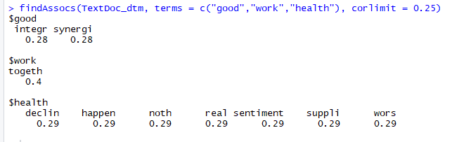 Figure 5.
Word association analysis for the top three most frequent terms
This script shows which words are most frequently associated with the top three terms (
Figure 5.
Word association analysis for the top three most frequent terms
This script shows which words are most frequently associated with the top three terms (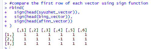 Figure 9.
Normalize scale and compare three vectors
Note the first element of each row (vector) is 1, indicating that all three methods have calculated a positive sentiment score, for the first response (line) in the text.
Emotion Classification
Emotion classification is built on the NRC Word-Emotion Association Lexicon (aka EmoLex).
The definition of “NRC Emotion Lexicon”, sourced from http://saifmohammad.com/WebPages/NRC-Emotion-Lexicon.htm is “The NRC Emotion Lexicon is a list of English words and their associations with eight basic emotions (anger, fear, anticipation, trust, surprise, sadness, joy, and disgust) and two sentiments (negative and positive).
The annotations were manually done by crowdsourcing.”
To understand this, explore the
Figure 9.
Normalize scale and compare three vectors
Note the first element of each row (vector) is 1, indicating that all three methods have calculated a positive sentiment score, for the first response (line) in the text.
Emotion Classification
Emotion classification is built on the NRC Word-Emotion Association Lexicon (aka EmoLex).
The definition of “NRC Emotion Lexicon”, sourced from http://saifmohammad.com/WebPages/NRC-Emotion-Lexicon.htm is “The NRC Emotion Lexicon is a list of English words and their associations with eight basic emotions (anger, fear, anticipation, trust, surprise, sadness, joy, and disgust) and two sentiments (negative and positive).
The annotations were manually done by crowdsourcing.”
To understand this, explore the