To run the code paste it into an R console window.
a <- 42
A <- a * 2  # R is case sensitive
print(a)
cat(A, "\n") # "84" is concatenated with "\n"
if(A>a) # true, 84 > 42
{
  cat(A, ">", a, "\n")
}
[1] 42
84
84 > 42
R uses <- for variable assignment.
Don't call your variables any of the following:
Howard Seltman provides more information about reserved terms in this "Learning R" lesson.
You can use underscores and periods in your identifiers. Google suggests tree.count for variables and DoSomething for functions.
Comments start with a # sign. Block Comments can't be be done nicely.
print() automatically appends a new line character to the output. With cat() you have to append it manually. print() can also show more types of content, such as functions:
print(cat)
> print(cat)
function (..., file = "", sep = " ", fill = FALSE, labels = NULL,
    append = FALSE)
{
    if (is.character(file))
        if (file == "")
  file <- stdout()
        else if (substring(file, 1L, 1L) == "|") {
  file <- pipe(substring(file, 2L), "w")
  on.exit(close(file))
        }
        else {
  file <- file(file, ifelse(append, "a", "w"))
  on.exit(close(file))
        }
    .Internal(cat(list(...), file, sep, fill, labels, append))
}
<environment: namespace:base>
You can get the documentation of a function from the R console if you type help(print).
If statements are quite straightforward:
if(condition)
{
	doSth()
}
Square <- function(x) {
  return(x^2)
}

print(Square(4))
print(Square(x=4)) # same thing
[1] 16
[1] 16
Functions can be defined like this: function(parameter1, parameter2, parameter3){code}.
For use they are assigned to a variable (using normal <- assignment operator).
The return function is used for return values: return(value). If no value is given NULL is returned.
Raise a to the power of b: a^b. It's also possible to use ** instead of ^.
Named arguments work like this: DoSomething(color="red",number=55).
You can also give the first arguments in order and then use named arguments: DoSth(value1,value2,arg4=value4,arg3=value3).
When using the console directly R automatically prints the return value of a statement if you don't assign it to a variable. This doesn't work in loops or functions.
You can use invisible(CalculateSth()) if you don't want the return value to be printed.
countdown <- function(from)
{
  print(from)
  while(from!=0)
  {
    Sys.sleep(1)
    from <- from - 1
    print(from)
  }
}

countdown(5)
> countdown(5)
[1] 5
[1] 4
[1] 3
[1] 2
[1] 1
[1] 0
Use while(condition){code}.
You can use the usual C-style operators: ==,<,||,&&,....
However, there are differences under some circumstances.
Suspends execution for the given amount of seconds.
readinteger <- function()
{
  n <- readline(prompt="Enter an integer: ")
  return(as.integer(n))
}

print(readinteger())
Enter an integer: 88
[1] 88
readline() lets the user enter a one-line string at the terminal.
The prompt argument is printed in front of the user input. It usually ends on ": ".
as.integer makes an integer out of the string.
Right now if the user doesn't enter an integer, as.integer will return NA (Not Available). We can avoid this by using is.na to check the user input and asking again if the value is NA:
readinteger <- function()
{
  n <- readline(prompt="Enter an integer: ")
  n <- as.integer(n)
  if (is.na(n)){
    n <- readinteger()
  }
  return(n)
}

print(readinteger())
Enter an integer:
Enter an integer: boo
Enter an integer: 44
[1] 44
Warning message:
In readinteger() : NAs introduced by coercion
However, a warning message is still shown. This is how to avoid it:
readinteger <- function()
{
  n <- readline(prompt="Enter an integer: ")
  if(!grepl("^[0-9]+$",n))
  {
    return(readinteger())
  }

  return(as.integer(n))
}

print(readinteger())
Enter an integer:
Enter an integer: 31r132weq
Enter an integer: effasdf
Enter an integer: 222
[1] 222
grepl returns TRUE if the regular expression "^[0-9]+$" is matched. (The expression checks for a string that consists of nothing but one or more digits.)
! negates the result and the if branch is executed if the user-entered string isn't an integer.
Use source("filename.r") to run this.
#utility functions

readinteger <- function()
{
  n <- readline(prompt="Enter an integer: ")
  if(!grepl("^[0-9]+$",n))
  {
    return(readinteger())
  }
  return(as.integer(n))
}

# real program start here

num <- round(runif(1) * 100, digits = 0)
guess <- -1

cat("Guess a number between 0 and 100.\n")

while(guess != num)
{
  guess <- readinteger()
  if (guess == num)
  {
    cat("Congratulations,", num, "is right.\n")
  }
  else if (guess < num)
  {
    cat("It's bigger!\n")
  }
  else if(guess > num)
  {
    cat("It's smaller!\n")
  }
}
> source("random-number-game.r")
Guess a number between 0 and 100.
Enter an integer: 50
It's smaller!
Enter an integer: 20
It's bigger!
Enter an integer: 40
It's bigger!
Enter an integer: 45
It's smaller!
Enter an integer: 43
It's bigger!
Enter an integer: 44
Congratulations, 44 is right.
The readinteger function has been explained in a previous example.
The round function rounds the first argument to the specified number of digits.
> round(22.5,0)  # rounds to even number
[1] 22
> round(3.14,1)
[1] 3.1
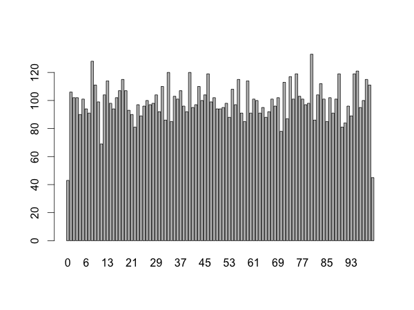
runif generates random numbers between 0 and 1.
The first argument specifies how many numbers you want.
runif(2)
[1] 0.8379240 0.1773677
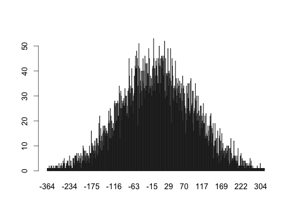
A non-uniform normal distribution would look like this:
sum(0:9)
append(LETTERS[1:13],letters[14:26])
c(1,6,4,9)*2
something <- c(1,4,letters[2])  # indices start at one, you get (1,4,"b")
length(something)
sum(0:9)
[1] 45
> append(LETTERS[1:13],letters[14:26])
 [1] "A" "B" "C" "D" "E" "F" "G" "H" "I" "J" "K" "L" "M" "n" "o"
[16] "p" "q" "r" "s" "t" "u" "v" "w" "x" "y" "z"
> c(1,6,4,9)*2
[1]  2 12  8 18
> something <- c(1,4,letters[2]) #indices start at one, you get (1,4,"b")
> length(something)
[1] 3
-5:5
[1] -5 -4 -3 -2 -1 0 1 2 3 4 5
The c function combines the parameters into a list and converts them to the same type.
c("test",3)
[1] "test" "3"
typeof("3")
[1] "character"Here 3 is converted to a string.
seq generates more complex regular sequences:
> seq(from=1,to=4,by=.6)
[1] 1.0 1.6 2.2 2.8 3.4 4.0
List members can be accessed using brackets as in most languages: (3:5)[2].
This returns 4 because indices start with 1.
You can also extract multiple list members from a list: letters[2:4] returns [1] "b" "c" "d".
You can use the append function for this.
Its return value has to be reassigned to the variable.
By default the new value is appended at the end of the list. You can use the after argument to change that:
a <- 1:4
append(a,2.4,after=2)
[1] 1.0 2.0 2.4 3.0 4.0
R allows you to easily operate on all list values at once.
c(1,2,3) + 3
This and the apply function allow you to avoid most for loops.
[1] 4 5 6
Lists for letters and month names are predefined:
letters
[1] "a" "b" "c" "d" "e" "f" "g" "h" "i" "j" "k" "l" "m" "n" "o"
[16] "p" "q" "r" "s" "t" "u" "v" "w" "x" "y" "z"
LETTERS
[1] "A" "B" "C" "D" "E" "F" "G" "H" "I" "J" "K" "L" "M" "N" "O"
[16] "P" "Q" "R" "S" "T" "U" "V" "W" "X" "Y" "Z"
month.abb
[1] "Jan" "Feb" "Mar" "Apr" "May" "Jun" "Jul" "Aug" "Sep" "Oct"
[11] "Nov" "Dec"
month.name
[1] "January"   "February"  "March"     "April"     "May"
 [6] "June"      "July"      "August"    "September" "October"
[11] "November"  "December"
Vectors are lists in which all elements have the same type. For example, the c function creates a vector.
This code uses a dataset file with population estimates by the US Census Bureau (more info).
tbl <- read.table(file.choose(),header=TRUE,sep=",")
population <- tbl["POPESTIMATE2009"]
print(summary(population[-1:-5,]))
    Min.  1st Qu.   Median     Mean  3rd Qu.     Max.
  544300  1734000  4141000  5980000  6613000 36960000
read.table can read a variety of basic data formats into tables or "data frames".
sep specifies the separator for the data, which is a comma for CSV files.
header indicates whether the first row contains the names of the data columns.
The first argument contains the file name.
In this case file.choose is used to show a dialog.
See the R documentation for more information.
You can use the column name as a string in brackets: tbl["POPESTIMATE2009"]:
   POPESTIMATE2009
1        307006550
2         55283679
3         66836911
[...]
Using the column number also works: tbl[17].
You can use the dollar sign for this: tbl$POPESTIMATE2009
[1] 307006550  55283679  66836911 113317879  71568081   4708708    698473
[8]   6595778   2889450  36961664   5024748   3518288    885122    599657
[...]
Here the table will be treated as a 2-dimensional matrix.
To get the first 5 rows from the population table:
population[1:5,] # first the rows, then the columns
[1] 307006550 55283679 66836911 113317879 71568081
The comma after the row information indicates that we want all columns. In this case we could also have written [1:5,1] because we only have 1 column in population.
Look at this data from the first 5 rows in the population column:
[1] 307006550 55283679 66836911 113317879 71568081
These are too big to be population values for US States.
They are the total US population and that of the US Census Bureau regions: Northeast, Midwest, South and West.
Since we are only interested in the states we can drop them like this:
population[-1:-5,]
Negative numbers in matrix indices can be used to omit specific rows or columns.
You can also fetch the population column at the same time as you remove the multi-state rows. Replace
population <- tbl["POPESTIMATE2009"]
print(summary(population[-1:-5,]))
with
print(summary(tbl[-1:-5,"POPESTIMATE2009"]))
summary calculates a few values based on the data passed as the first argument. The exact values calculated depend on the class of the data.
summary(1:10)
   Min. 1st Qu.  Median    Mean 3rd Qu.    Max.
   1.00    3.25    5.50    5.50    7.75   10.00
This code uses a dataset file with population estimates by the US Census Bureau (more info).
tbl <- read.table(file.choose(),header=TRUE,sep=',')
population <- tbl[c("NAME","POPESTIMATE2009","NPOPCHG_2009")]
smallest.state.pop <- min(population$POPESTIMATE2009)
print(population[population$POPESTIMATE2009==smallest.state.pop,])
      NAME POPESTIMATE2009 NPOPCHG_2009
56 Wyoming          544270        11289
This piece of code extracts the data about the smallest state from the data frame.
The first line has reads the data from the CSV file (as explained here).
The second line limits the rows to the state name, the population estimate for 2009 and the total population change for 2009.
Let's use the head function to look at what we get:
head(population)
 NAME POPESTIMATE2009 NPOPCHG_2009
1 United States       307006550      2631704
2     Northeast        55283679       223483
3       Midwest        66836911       241314
4         South       113317879      1296857
5          West        71568081       870050
6       Alabama         4708708        31244
First the POPESTIMATE2009 column is selected:
population$POPESTIMATE2009
 [1] 307006550  55283679  66836911 113317879  71568081   4708708    698473
 [8]   6595778   2889450  36961664   5024748   3518288    885122    599657
[...]
[50]   2784572    621760   7882590   6664195   1819777   5654774    544270
[57]   3967288
Then the min function is used to find the minimum:
min(population$POPESTIMATE2009)
[1] 544270
You use something like a WHERE clause in data frame indices:
data.frame[condition]This condition works because it creates an array of booleans depending on whether the field value is a match:
population$POPESTIMATE2009==smallest.state.pop
[1] FALSE FALSE FALSE FALSE FALSE FALSE FALSE FALSE FALSE FALSE FALSE FALSE
[13] FALSE FALSE FALSE FALSE FALSE FALSE FALSE FALSE FALSE FALSE FALSE FALSE
[25] FALSE FALSE FALSE FALSE FALSE FALSE FALSE FALSE FALSE FALSE FALSE FALSE
[37] FALSE FALSE FALSE FALSE FALSE FALSE FALSE FALSE FALSE FALSE FALSE FALSE
[49] FALSE FALSE FALSE FALSE FALSE FALSE FALSE  TRUE FALSE
In this case only the second to last row should be selected. We use a comma after the row index because we want all the columns:
population[population$POPESTIMATE2009==smallest.state.pop,]
      NAME POPESTIMATE2009 NPOPCHG_2009
56 Wyoming          544270        11289
I find it easiest to use RStudio. You can also paste the code in a normal R console or let R run a source file. However these approaches are a bit less fail-safe.
Download and install RStudio.
Open RStudio and do this:
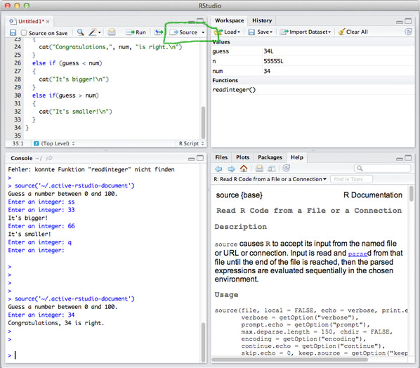
You can also use the console in RStudio. If you click "Run" instead of "Source" user input might not work properly.
You can use the R documentation like this: help(function.name).
This will generally work if you use source("filename.r") to run your code. If you paste the code some of it might be read as user input.
You can run a source file like this: r -f filename.r.
R also provides a lot of other command line arguments.
I have not managed to get user input to work here.
Here are a few data sets to play around with.
print(head(mtcars))
         mpg cyl disp  hp drat    wt  qsec vs am gear carb
Mazda RX4         21.0   6  160 110 3.90 2.620 16.46  0  1    4    4
Mazda RX4 Wag     21.0   6  160 110 3.90 2.875 17.02  0  1    4    4
Datsun 710        22.8   4  108  93 3.85 2.320 18.61  1  1    4    1
Hornet 4 Drive    21.4   6  258 110 3.08 3.215 19.44  1  0    3    1
Hornet Sportabout 18.7   8  360 175 3.15 3.440 17.02  0  0    3    2
Valiant           18.1   6  225 105 2.76 3.460 20.22  1  0    3    1
This is a built-in data set. Use it for sorting, filtering etc.
You can use matrix to generate a quick dataset. The first argument must contain your data. You can use a distribution function or sample for it.
print(matrix(runif(6*3), nrow=6, ncol=3))
[,1]       [,2]       [,3]
[1,] 0.94210093 0.23582446 0.19571104
[2,] 0.45026399 0.77989358 0.69763985
[3,] 0.03567169 0.40572983 0.83394039
[4,] 0.31246289 0.08076585 0.74957412
[5,] 0.61316957 0.94886782 0.90769685
[6,] 0.94545758 0.48658449 0.03396954
The US government published data sets on data.gov. This includes US census data. Most files are in CSV format and you can use read.table to read them.
The UN publishes data at data.un.org. This data is also available in CSV format.