#==============
# LOAD PACKAGES
#==============
library(tidyverse)
library(sf)
library(rvest)
library(stringr)
library(scales)
#library(viridis)
#============
# SCRAPE DATA
#============
df.oil <- read_html("https://en.wikipedia.org/wiki/List_of_countries_by_oil_production") %>%
html_nodes("table") %>%
.[[1]] %>%
html_table()
#====================
# CHANGE COLUMN NAMES
#====================
colnames(df.oil) <- c('rank', 'country', 'oil_bbl_per_day')
#=============================
# WRANGLE VARIABLES INTO SHAPE
#=============================
#----------------------------------
# COERCE 'rank' VARIABLE TO INTEGER
#----------------------------------
df.oil <- df.oil %>% mutate(rank = as.integer(rank))
df.oil %>% glimpse()
#---------------------------------------------------
# WRANGLE FROM CHARACTER TO NUMERIC: oil_bbl_per_day
#---------------------------------------------------
df.oil <- df.oil %>% mutate(oil_bbl_per_day = oil_bbl_per_day %>% str_replace_all(',','') %>% as.integer())
# inspect
df.oil %>% glimpse()
#===========================
#CREATE VARIABLE: 'opec_ind'
#===========================
df.oil <- df.oil %>% mutate(opec_ind = if_else(str_detect(country, 'OPEC'), 1, 0))
#=========================================================
# CLEAN UP 'country'
# - some country names are tagged as being OPEC countries
# and this information is in the country name
# - we will strip this information out
#=========================================================
df.oil <- df.oil %>% mutate(country = country %>% str_replace(' \\(OPEC\\)', '') %>% str_replace('\\s{2,}',' '))
# inspect
df.oil %>% glimpse()
#------------------------------------------
# EXAMINE OPEC COUNTRIES
# - here, we'll just visually inspect
# to make sure that the names are correct
#------------------------------------------
df.oil %>%
filter(opec_ind == 1) %>%
select(country)
#==================
# REORDER VARIABLES
#==================
df.oil <- df.oil %>% select(rank, country, opec_ind, oil_bbl_per_day)
df.oil %>% glimpse()
#========
# GET MAP
#========
map.world <- map_data('world')
df.oil
#==========================
# CHECK FOR JOIN MISMATCHES
#==========================
anti_join(df.oil, map.world, by = c('country' = 'region'))
# rank country opec_ind oil_bbl_per_day
# 1 67 Congo, Democratic Republic of the 0 20,000
# 2 47 Trinidad and Tobago 0 60,090
# 3 34 Sudan and South Sudan 0 255,000
# 4 30 Congo, Republic of the 0 308,363
# 5 20 United Kingdom 0 939,760
# 6 3 United States 0 8,875,817
#=====================
# RECODE COUNTRY NAMES
#=====================
map.world %>%
group_by(region) %>%
summarise() %>%
print(n = Inf)
# UK
# USA
# Democratic Republic of the Congo
# Trinidad
# Sudan
# South Sudan
df.oil <- df.oil %>% mutate(country = recode(country, `United States` = 'USA'
, `United Kingdom` = 'UK'
, `Congo, Democratic Republic of the` = 'Democratic Republic of the Congo'
, `Trinidad and Tobago` = 'Trinidad'
, `Sudan and South Sudan` = 'Sudan'
#, `Sudan and South Sudan` = 'South Sudan'
, `Congo, Republic of the` = 'Republic of Congo'
)
)
#-----------------------
# JOIN DATASETS TOGETHER
#-----------------------
map.oil <- left_join( map.world, df.oil, by = c('region' = 'country'))
#=====
# PLOT
#=====
# BASIC (this is a first draft)
ggplot(map.oil, aes( x = long, y = lat, group = group )) +
geom_polygon(aes(fill = oil_bbl_per_day))
#=======================
# FINAL, FORMATTED DRAFT
#=======================
df.oil %>% filter(oil_bbl_per_day > 822675) %>% summarise(mean(oil_bbl_per_day))
# 3190373
df.oil %>% filter(oil_bbl_per_day < 822675) %>% summarise(mean(oil_bbl_per_day))
# 96581.08
ggplot(map.oil, aes( x = long, y = lat, group = group )) +
geom_polygon(aes(fill = oil_bbl_per_day)) +
scale_fill_gradientn(colours = c('#461863','#404E88','#2A8A8C','#7FD157','#F9E53F')
,values = scales::rescale(c(100,96581,822675,3190373,10000000))
,labels = comma
,breaks = c(100,96581,822675,3190373,10000000)
) +
guides(fill = guide_legend(reverse = T)) +
labs(fill = 'bbl/day'
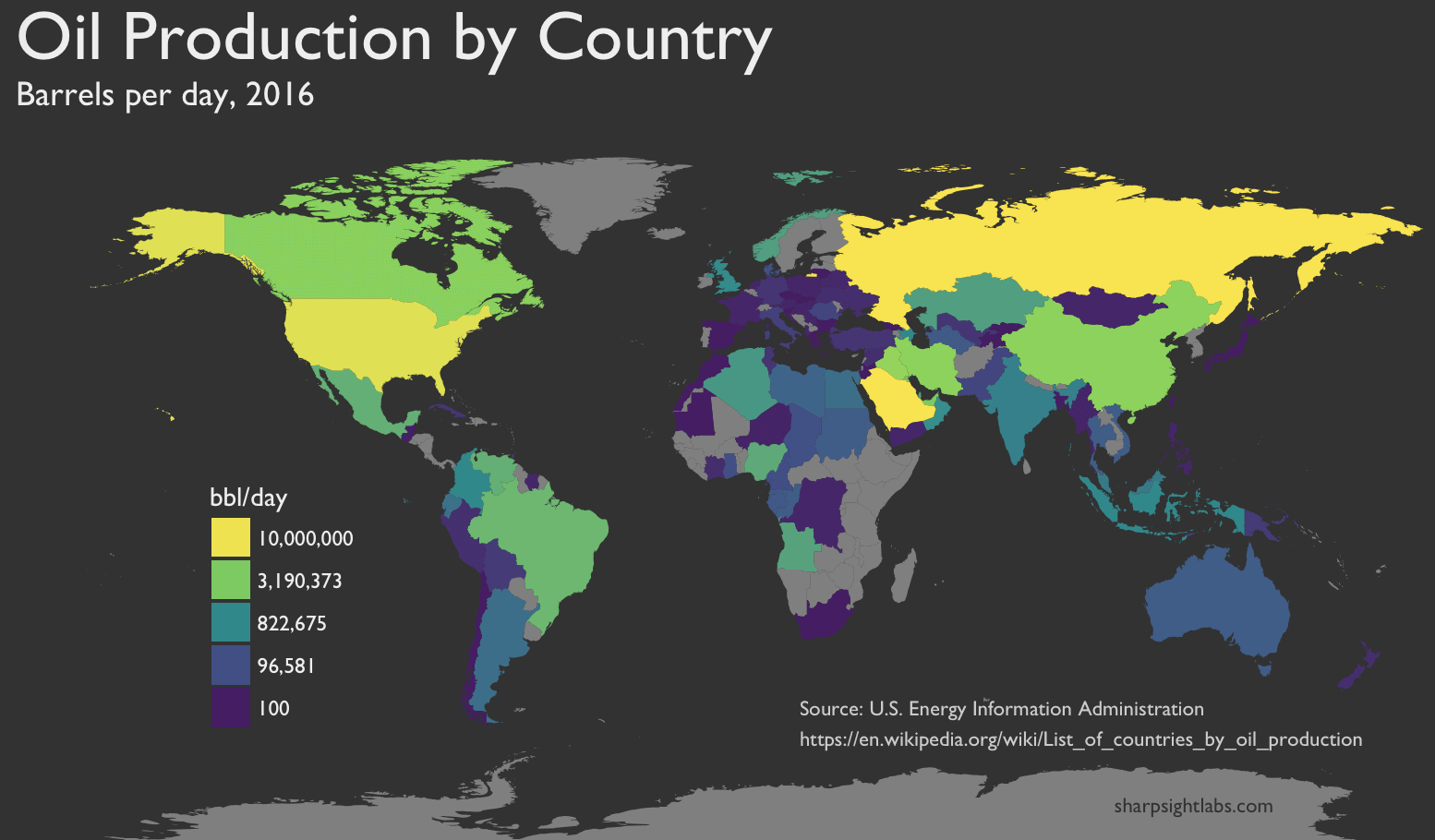
,title = 'Oil Production by Country'
,subtitle = 'Barrels per day, 2016'
,x = NULL
,y = NULL) +
theme(text = element_text(family = 'Gill Sans', color = '#EEEEEE')
,plot.title = element_text(size = 28)
,plot.subtitle = element_text(size = 14)
,axis.ticks = element_blank()
,axis.text = element_blank()
,panel.grid = element_blank()
,panel.background = element_rect(fill = '#333333')
,plot.background = element_rect(fill = '#333333')
,legend.position = c(.18,.36)
,legend.background = element_blank()
,legend.key = element_blank()
) +
annotate(geom = 'text'
,label = 'Source: U.S. Energy Information Administration\nhttps://en.wikipedia.org/wiki/List_of_countries_by_oil_production'
,x = 18, y = -55
,size = 3
,family = 'Gill Sans'
,color = '#CCCCCC'
,hjust = 'left'
)
And here’s the finalized map that the code produces: