| Prometheus | 2 | Adventure,Mystery,Sci-Fi | Following clues to the origin of mankind, a te... | Ridley Scott | Noomi Rapace, Logan Marshall-Green, Michael Fa... | 2012 | 124 | 7.0 | 485820 | 126.46 | 65.0 | bad |
|---|
| The Martian | 103 | Adventure,Drama,Sci-Fi | An astronaut becomes stranded on Mars after hi... | Ridley Scott | Matt Damon, Jessica Chastain, Kristen Wiig, Ka... | 2015 | 144 | 8.0 | 556097 | 228.43 | 80.0 | good |
|---|
| Robin Hood | 388 | Action,Adventure,Drama | In 12th century England, Robin and his band of... | Ridley Scott | Russell Crowe, Cate Blanchett, Matthew Macfady... | 2010 | 140 | 6.7 | 221117 | 105.22 | 53.0 | bad |
|---|
| American Gangster | 471 | Biography,Crime,Drama | In 1970s America, a detective works to bring d... | Ridley Scott | Denzel Washington, Russell Crowe, Chiwetel Eji... | 2007 | 157 | 7.8 | 337835 | 130.13 | 76.0 | bad |
|---|
| Exodus: Gods and Kings | 517 | Action,Adventure,Drama | The defiant leader Moses rises up against the ... | Ridley Scott | Christian Bale, Joel Edgerton, Ben Kingsley, S... | 2014 | 150 | 6.0 | 137299 | 65.01 | 52.0 | bad |
|---|
 What's with the semicolon? It's not a syntax error, just a way to hide the
  gives us on the ratings column:
movies_df['rating'].describe()
Out:
count 1000.000000
mean 6.723200
std 0.945429
min 1.900000
25% 6.200000
50% 6.800000
75% 7.400000
max 9.000000
Name: rating, dtype: float64
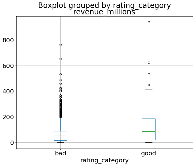
Using a Boxplot we can visualize this data:
movies_df['rating'].plot(kind="box");
RESULT:
gives us on the ratings column:
movies_df['rating'].describe()
Out:
count 1000.000000
mean 6.723200
std 0.945429
min 1.900000
25% 6.200000
50% 6.800000
75% 7.400000
max 9.000000
Name: rating, dtype: float64
Using a Boxplot we can visualize this data:
movies_df['rating'].plot(kind="box");
RESULT:


 for more information on what it can do.