D3 API Reference
Must Watch!
MustWatch
D3 4.0 is a collection of modules that are designed to work together; you can use the modules independently, or you can use them together as part of the default build.
The source and documentation for each module is available in its repository.
Follow the links below to learn more.
For changes between 3.x and 4.0, see CHANGES; see also the 3.x reference.
d3-array
Data in JavaScript is often represented by an iterable (such as an array, set or generator), and so iterable manipulation is a common task when analyzing or visualizing data.
For example, you might take a contiguous slice (subset) of an array, filter an array using a predicate function, or map an array to a parallel set of values using a transform function.
Before looking at the methods that d3-array provides, familiarize yourself with the powerful array methods built-in to JavaScript.
JavaScript includes mutation methods that modify the array:
array.pop - Remove the last element from the array.
array.push - Add one or more elements to the end of the array.
array.reverse - Reverse the order of the elements of the array.
array.shift - Remove the first element from the array.
array.sort - Sort the elements of the array.
array.splice - Add or remove elements from the array.
array.unshift - Add one or more elements to the front of the array.
There are also access methods that return some representation of the array:
array.concat - Join the array with other array(s) or value(s).
array.join - Join all elements of the array into a string.
array.slice - Extract a section of the array.
array.indexOf - Find the first occurrence of a value within the array.
array.lastIndexOf - Find the last occurrence of a value within the array.
And finally iteration methods that apply functions to elements in the array:
array.filter - Create a new array with only the elements for which a predicate is true.
array.forEach - Call a function for each element in the array.
array.every - See if every element in the array satisfies a predicate.
array.map - Create a new array with the result of calling a function on every element in the array.
array.some - See if at least one element in the array satisfies a predicate.
array.reduce - Apply a function to reduce the array to a single value (from left-to-right).
array.reduceRight - Apply a function to reduce the array to a single value (from right-to-left).
Installing
If you use NPM, npm install d3-array.
Otherwise, download the latest release.
You can also load directly from d3js.org, either as a standalone library or as part of D3.
AMD, CommonJS, and vanilla environments are supported.
In vanilla, a d3 global is exported:
<script src="https://d3js.org/d3-array.v2.min.js"></script>
<script>
var min = d3.min(array);
</script>
API Reference
Statistics
Search
Transformations
Iterables
Sets
Bins
Statistics
Methods for computing basic summary statistics.
# d3.min(iterable[, accessor]) · Source, Examples
Returns the minimum value in the given iterable using natural order.
If the iterable contains no comparable values, returns undefined.
An optional accessor function may be specified, which is equivalent to calling Array.from before computing the minimum value.
Unlike the built-in Math.min, this method ignores undefined, null and NaN values; this is useful for ignoring missing data.
In addition, elements are compared using natural order rather than numeric order.
For example, the minimum of the strings [“20”, “3”] is “20”, while the minimum of the numbers [20, 3] is 3.
See also extent.
# d3.minIndex(iterable[, accessor]) · Source, Examples
Returns the index of the minimum value in the given iterable using natural order.
If the iterable contains no comparable values, returns -1.
An optional accessor function may be specified, which is equivalent to calling Array.from before computing the minimum value.
Unlike the built-in Math.min, this method ignores undefined, null and NaN values; this is useful for ignoring missing data.
In addition, elements are compared using natural order rather than numeric order.
For example, the minimum of the strings [“20”, “3”] is “20”, while the minimum of the numbers [20, 3] is 3.
# d3.max(iterable[, accessor]) · Source, Examples
Returns the maximum value in the given iterable using natural order.
If the iterable contains no comparable values, returns undefined.
An optional accessor function may be specified, which is equivalent to calling Array.from before computing the maximum value.
Unlike the built-in Math.max, this method ignores undefined values; this is useful for ignoring missing data.
In addition, elements are compared using natural order rather than numeric order.
For example, the maximum of the strings [“20”, “3”] is “3”, while the maximum of the numbers [20, 3] is 20.
See also extent.
# d3.maxIndex(iterable[, accessor]) · Source, Examples
Returns the index of the maximum value in the given iterable using natural order.
If the iterable contains no comparable values, returns -1.
An optional accessor function may be specified, which is equivalent to calling Array.from before computing the maximum value.
Unlike the built-in Math.max, this method ignores undefined values; this is useful for ignoring missing data.
In addition, elements are compared using natural order rather than numeric order.
For example, the maximum of the strings [“20”, “3”] is “3”, while the maximum of the numbers [20, 3] is 20.
# d3.extent(iterable[, accessor]) · Source, Examples
Returns the minimum and maximum value in the given iterable using natural order.
If the iterable contains no comparable values, returns [undefined, undefined].
An optional accessor function may be specified, which is equivalent to calling Array.from before computing the extent.
# d3.sum(iterable[, accessor]) · Source, Examples
Returns the sum of the given iterable of numbers.
If the iterable contains no numbers, returns 0.
An optional accessor function may be specified, which is equivalent to calling Array.from before computing the sum.
This method ignores undefined and NaN values; this is useful for ignoring missing data.
# d3.mean(iterable[, accessor]) · Source, Examples
Returns the mean of the given iterable of numbers.
If the iterable contains no numbers, returns undefined.
An optional accessor function may be specified, which is equivalent to calling Array.from before computing the mean.
This method ignores undefined and NaN values; this is useful for ignoring missing data.
# d3.median(iterable[, accessor]) · Source, Examples
Returns the median of the given iterable of numbers using the R-7 method.
If the iterable contains no numbers, returns undefined.
An optional accessor function may be specified, which is equivalent to calling Array.from before computing the median.
This method ignores undefined and NaN values; this is useful for ignoring missing data.
# d3.cumsum(iterable[, accessor]) · Source, Examples
Returns the cumulative sum of the given iterable of numbers, as a Float64Array of the same length.
If the iterable contains no numbers, returns zeros.
An optional accessor function may be specified, which is equivalent to calling Array.from before computing the cumulative sum.
This method ignores undefined and NaN values; this is useful for ignoring missing data.
# d3.quantile(iterable, p[, accessor]) · Source, Examples
Returns the p-quantile of the given iterable of numbers, where p is a number in the range [0, 1].
For example, the median can be computed using p = 0.5, the first quartile at p = 0.25, and the third quartile at p = 0.75.
This particular implementation uses the R-7 method, which is the default for the R programming language and Excel.
For example:
var a = [0, 10, 30];
d3.quantile(a, 0); // 0
d3.quantile(a, 0.5); // 10
d3.quantile(a, 1); // 30
d3.quantile(a, 0.25); // 5
d3.quantile(a, 0.75); // 20
d3.quantile(a, 0.1); // 2
An optional accessor function may be specified, which is equivalent to calling array.map(accessor) before computing the quantile.
# d3.quantileSorted(array, p[, accessor]) · Source, Examples
Similar to quantile, but expects the input to be a sorted array of values.
In contrast with quantile, the accessor is only called on the elements needed to compute the quantile.
# d3.variance(iterable[, accessor]) · Source, Examples
Returns an unbiased estimator of the population variance of the given iterable of numbers using Welford’s algorithm.
If the iterable has fewer than two numbers, returns undefined.
An optional accessor function may be specified, which is equivalent to calling Array.from before computing the variance.
This method ignores undefined and NaN values; this is useful for ignoring missing data.
# d3.deviation(iterable[, accessor]) · Source, Examples
Returns the standard deviation, defined as the square root of the bias-corrected variance, of the given iterable of numbers.
If the iterable has fewer than two numbers, returns undefined.
An optional accessor function may be specified, which is equivalent to calling Array.from before computing the standard deviation.
This method ignores undefined and NaN values; this is useful for ignoring missing data.
# d3.fsum([values][, accessor]) · Source, Examples
Returns a full precision summation of the given values.
d3.fsum([.1, .1, .1, .1, .1, .1, .1, .1, .1, .1]); // 1
d3.sum([.1, .1, .1, .1, .1, .1, .1, .1, .1, .1]); // 0.9999999999999999
Although slower, d3.fsum can replace d3.sum wherever greater precision is needed.
Uses d3.Adder.
# new d3.Adder()
Creates a full precision adder for IEEE 754 floating point numbers, setting its initial value to 0.
# adder.add(number)
Adds the specified number to the adder’s current value and returns the adder.
# adder.valueOf()
Returns the IEEE 754 double precision representation of the adder’s current value.
Most useful as the short-hand notation +adder.
Search
Methods for searching arrays for a specific element.
# d3.least(iterable[, comparator]) · Source, Examples
# d3.least(iterable[, accessor])
Returns the least element of the specified iterable according to the specified comparator or accessor.
If the given iterable contains no comparable elements (i.e., the comparator returns NaN when comparing each element to itself), returns undefined.
If comparator is not specified, it defaults to ascending.
For example:
const array = [{foo: 42}, {foo: 91}];
d3.least(array, (a, b) => a.foo - b.foo); // {foo: 42}
d3.least(array, (a, b) => b.foo - a.foo); // {foo: 91}
d3.least(array, a => a.foo); // {foo: 42}
This function is similar to min, except it allows the use of a comparator rather than an accessor.
# d3.leastIndex(iterable[, comparator]) · Source, Examples
# d3.leastIndex(iterable[, accessor])
Returns the index of the least element of the specified iterable according to the specified comparator or accessor.
If the given iterable contains no comparable elements (i.e., the comparator returns NaN when comparing each element to itself), returns -1.
If comparator is not specified, it defaults to ascending.
For example:
const array = [{foo: 42}, {foo: 91}];
d3.leastIndex(array, (a, b) => a.foo - b.foo); // 0
d3.leastIndex(array, (a, b) => b.foo - a.foo); // 1
d3.leastIndex(array, a => a.foo); // 0
This function is similar to minIndex, except it allows the use of a comparator rather than an accessor.
# d3.greatest(iterable[, comparator]) · Source, Examples
# d3.greatest(iterable[, accessor])
Returns the greatest element of the specified iterable according to the specified comparator or accessor.
If the given iterable contains no comparable elements (i.e., the comparator returns NaN when comparing each element to itself), returns undefined.
If comparator is not specified, it defaults to ascending.
For example:
const array = [{foo: 42}, {foo: 91}];
d3.greatest(array, (a, b) => a.foo - b.foo); // {foo: 91}
d3.greatest(array, (a, b) => b.foo - a.foo); // {foo: 42}
d3.greatest(array, a => a.foo); // {foo: 91}
This function is similar to max, except it allows the use of a comparator rather than an accessor.
# d3.greatestIndex(iterable[, comparator]) · Source, Examples
# d3.greatestIndex(iterable[, accessor])
Returns the index of the greatest element of the specified iterable according to the specified comparator or accessor.
If the given iterable contains no comparable elements (i.e., the comparator returns NaN when comparing each element to itself), returns -1.
If comparator is not specified, it defaults to ascending.
For example:
const array = [{foo: 42}, {foo: 91}];
d3.greatestIndex(array, (a, b) => a.foo - b.foo); // 1
d3.greatestIndex(array, (a, b) => b.foo - a.foo); // 0
d3.greatestIndex(array, a => a.foo); // 1
This function is similar to maxIndex, except it allows the use of a comparator rather than an accessor.
# d3.bisectLeft(array, x[, lo[, hi]]) · Source
Returns the insertion point for x in array to maintain sorted order.
The arguments lo and hi may be used to specify a subset of the array which should be considered; by default the entire array is used.
If x is already present in array, the insertion point will be before (to the left of) any existing entries.
The return value is suitable for use as the first argument to splice assuming that array is already sorted.
The returned insertion point i partitions the array into two halves so that all v < x for v in array.slice(lo, i) for the left side and all v >= x for v in array.slice(i, hi) for the right side.
# d3.bisect(array, x[, lo[, hi]]) · Source, Examples
# d3.bisectRight(array, x[, lo[, hi]])
Similar to bisectLeft, but returns an insertion point which comes after (to the right of) any existing entries of x in array.
The returned insertion point i partitions the array into two halves so that all v <= x for v in array.slice(lo, i) for the left side and all v > x for v in array.slice(i, hi) for the right side.
# d3.bisectCenter(array, x[, lo[, hi]]) · Source, Examples
Returns the index of the value closest to x in the given array of numbers.
The arguments lo (inclusive) and hi (exclusive) may be used to specify a subset of the array which should be considered; by default the entire array is used.
See bisector.center.
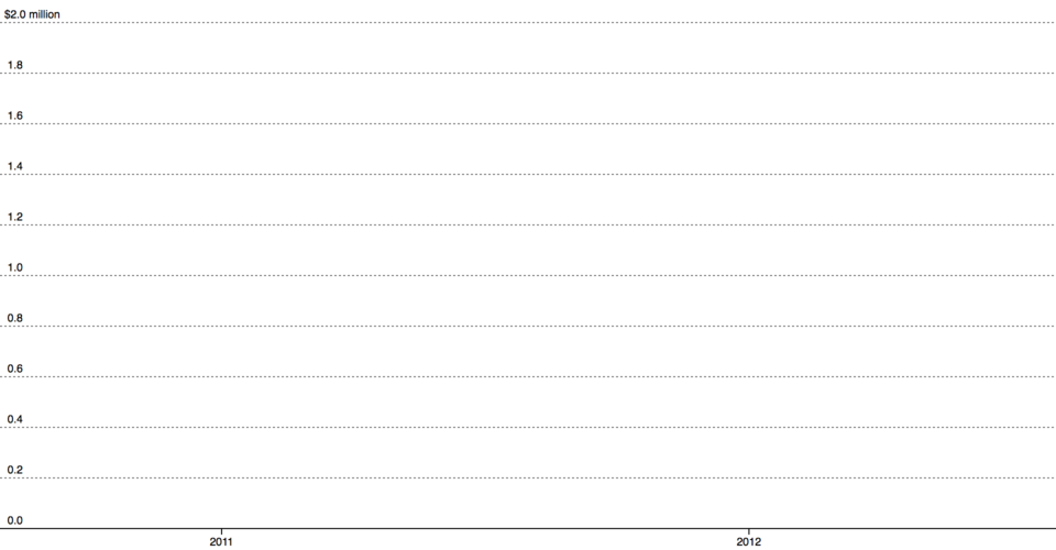
# d3.bisector(accessor) · Source
# d3.bisector(comparator)
Returns a new bisector using the specified accessor or comparator function.
This method can be used to bisect arrays of objects instead of being limited to simple arrays of primitives.
For example, given the following array of objects:
var data = [
{date: new Date(2011, 1, 1), value: 0.5},
{date: new Date(2011, 2, 1), value: 0.6},
{date: new Date(2011, 3, 1), value: 0.7},
{date: new Date(2011, 4, 1), value: 0.8}
];
A suitable bisect function could be constructed as:
var bisectDate = d3.bisector(function(d) { return d.date; }).right;
This is equivalent to specifying a comparator:
var bisectDate = d3.bisector(function(d, x) { return d.date - x; }).right;
And then applied as bisectDate(array, date), returning an index.
Note that the comparator is always passed the search value x as the second argument.
Use a comparator rather than an accessor if you want values to be sorted in an order different than natural order, such as in descending rather than ascending order.
# bisector.left(array, x[, lo[, hi]]) · Source
Equivalent to bisectLeft, but uses this bisector’s associated comparator.
# bisector.right(array, x[, lo[, hi]]) · Source
Equivalent to bisectRight, but uses this bisector’s associated comparator.
# bisector.center(array, x[, lo[, hi]]) · Source
Returns the index of the closest value to x in the given sorted array.
This expects that the bisector’s associated accessor returns a quantitative value, or that the bisector’s associated comparator returns a signed distance; otherwise, this method is equivalent to bisector.left.
# d3.quickselect(array, k, left = 0, right = array.length - 1, compare = ascending) · Source, Examples
See mourner/quickselect.
# d3.ascending(a, b) · Source, Examples
Returns -1 if a is less than b, or 1 if a is greater than b, or 0.
This is the comparator function for natural order, and can be used in conjunction with the built-in array.sort method to arrange elements in ascending order.
It is implemented as:
function ascending(a, b) {
return a < b ? -1 : a > b ? 1 : a >= b ? 0 : NaN;
}
Note that if no comparator function is specified to the built-in sort method, the default order is lexicographic (alphabetical), not natural! This can lead to surprising behavior when sorting an array of numbers.
# d3.descending(a, b) · Source, Examples
Returns -1 if a is greater than b, or 1 if a is less than b, or 0.
This is the comparator function for reverse natural order, and can be used in conjunction with the built-in array sort method to arrange elements in descending order.
It is implemented as:
function descending(a, b) {
return b < a ? -1 : b > a ? 1 : b >= a ? 0 : NaN;
}
Note that if no comparator function is specified to the built-in sort method, the default order is lexicographic (alphabetical), not natural! This can lead to surprising behavior when sorting an array of numbers.
Transformations
Methods for transforming arrays and for generating new arrays.
# d3.group(iterable, ...keys) · Source, Examples
Groups the specified iterable of values into a Map from key to array of value.
For example, given some data:
data = [
{name: "jim", amount: "34.0", date: "11/12/2015"},
{name: "carl", amount: "120.11", date: "11/12/2015"},
{name: "stacy", amount: "12.01", date: "01/04/2016"},
{name: "stacy", amount: "34.05", date: "01/04/2016"}
]
To group the data by name:
d3.group(data, d => d.name)
This produces:
Map(3) {
"jim" => Array(1)
"carl" => Array(1)
"stacy" => Array(2)
}
If more than one key is specified, a nested Map is returned.
For example:
d3.group(data, d => d.name, d => d.date)
This produces:
Map(3) {
"jim" => Map(1) {
"11/12/2015" => Array(1)
}
"carl" => Map(1) {
"11/12/2015" => Array(1)
}
"stacy" => Map(1) {
"01/04/2016" => Array(2)
}
}
To convert a Map to an Array, use Array.from.
For example:
Array.from(d3.group(data, d => d.name))
This produces:
[
["jim", Array(1)],
["carl", Array(1)],
["stacy", Array(2)]
]
You can also simultaneously convert the [key, value] to some other representation by passing a map function to Array.from:
Array.from(d3.group(data, d => d.name), ([key, value]) => ({key, value}))
This produces:
[
{key: "jim", value: Array(1)},
{key: "carl", value: Array(1)},
{key: "stacy", value: Array(2)}
]
In the near future, selection.data will accept iterables directly, meaning that you can use a Map (or Set or other iterable) to perform a data join without first needing to convert to an array.
# d3.groups(iterable, ...keys) · Source, Examples
Equivalent to group, but returns nested arrays instead of nested maps.
# d3.index(iterable, ...keys) · Source
Equivalent to group but returns a unique value per compound key instead of an array, throwing if the key is not unique.
For example, given the data defined above,
d3.index(data, d => d.amount)
returns
Map(4) {
"34.0" => Object {name: "jim", amount: "34.0", date: "11/12/2015"}
"120.11" => Object {name: "carl", amount: "120.11", date: "11/12/2015"}
"12.01" => Object {name: "stacy", amount: "12.01", date: "01/04/2016"}
"34.05" => Object {name: "stacy", amount: "34.05", date: "01/04/2016"}
}
On the other hand,
d3.index(data, d => d.name)
throws an error because two objects share the same name.
# d3.indexes(iterable, ...keys) · Source
Equivalent to index, but returns nested arrays instead of nested maps.
# d3.rollup(iterable, reduce, ...keys) · Source, Examples
Groups and reduces the specified iterable of values into a Map from key to value.
For example, given some data:
data = [
{name: "jim", amount: "34.0", date: "11/12/2015"},
{name: "carl", amount: "120.11", date: "11/12/2015"},
{name: "stacy", amount: "12.01", date: "01/04/2016"},
{name: "stacy", amount: "34.05", date: "01/04/2016"}
]
To count the number of elements by name:
d3.rollup(data, v => v.length, d => d.name)
This produces:
Map(3) {
"jim" => 1
"carl" => 1
"stacy" => 2
}
If more than one key is specified, a nested Map is returned.
For example:
d3.rollup(data, v => v.length, d => d.name, d => d.date)
This produces:
Map(3) {
"jim" => Map(1) {
"11/12/2015" => 1
}
"carl" => Map(1) {
"11/12/2015" => 1
}
"stacy" => Map(1) {
"01/04/2016" => 2
}
}
To convert a Map to an Array, use Array.from.
See d3.group for examples.
# d3.rollups(iterable, ...keys) · Source, Examples
Equivalent to rollup, but returns nested arrays instead of nested maps.
# d3.count(iterable[, accessor]) · Source, Examples
Returns the number of valid number values (i.e., not null, NaN, or undefined) in the specified iterable; accepts an accessor.
For example:
d3.count([{n: "Alice", age: NaN}, {n: "Bob", age: 18}, {n: "Other"}], d => d.age) // 1
# d3.cross(...iterables[, reducer]) · Source, Examples
Returns the Cartesian product of the specified iterables.
For example, if two iterables a and b are specified, for each element i in the iterable a and each element j in the iterable b, in order, invokes the specified reducer function passing the element i and element j.
If a reducer is not specified, it defaults to a function which creates a two-element array for each pair:
function pair(a, b) {
return [a, b];
}
For example:
d3.cross([1, 2], ["x", "y"]); // returns [[1, "x"], [1, "y"], [2, "x"], [2, "y"]]
d3.cross([1, 2], ["x", "y"], (a, b) => a + b); // returns ["1x", "1y", "2x", "2y"]
# d3.merge(iterables) · Source, Examples
Merges the specified iterable of iterables into a single array.
This method is similar to the built-in array concat method; the only difference is that it is more convenient when you have an array of arrays.
d3.merge([[1], [2, 3]]); // returns [1, 2, 3]
# d3.pairs(iterable[, reducer]) · Source, Examples
For each adjacent pair of elements in the specified iterable, in order, invokes the specified reducer function passing the element i and element i - 1.
If a reducer is not specified, it defaults to a function which creates a two-element array for each pair:
function pair(a, b) {
return [a, b];
}
For example:
d3.pairs([1, 2, 3, 4]); // returns [[1, 2], [2, 3], [3, 4]]
d3.pairs([1, 2, 3, 4], (a, b) => b - a); // returns [1, 1, 1];
If the specified iterable has fewer than two elements, returns the empty array.
# d3.permute(source, keys) · Source, Examples
Returns a permutation of the specified source object (or array) using the specified iterable of keys.
The returned array contains the corresponding property of the source object for each key in keys, in order.
For example:
permute(["a", "b", "c"], [1, 2, 0]); // returns ["b", "c", "a"]
It is acceptable to have more keys than source elements, and for keys to be duplicated or omitted.
This method can also be used to extract the values from an object into an array with a stable order.
Extracting keyed values in order can be useful for generating data arrays in nested selections.
For example:
let object = {yield: 27, variety: "Manchuria", year: 1931, site: "University Farm"};
let fields = ["site", "variety", "yield"];
d3.permute(object, fields); // returns ["University Farm", "Manchuria", 27]
# d3.shuffle(array[, start[, stop]]) · Source, Examples
Randomizes the order of the specified array in-place using the Fisher–Yates shuffle and returns the array.
If start is specified, it is the starting index (inclusive) of the array to shuffle; if start is not specified, it defaults to zero.
If stop is specified, it is the ending index (exclusive) of the array to shuffle; if stop is not specified, it defaults to array.length.
For example, to shuffle the first ten elements of the array: shuffle(array, 0, 10).
# d3.shuffler(random) · Source
Returns a shuffle function given the specified random source.
For example, using d3.randomLcg:
const random = d3.randomLcg(0.9051667019185816);
const shuffle = d3.shuffler(random);
shuffle([0, 1, 2, 3, 4, 5, 6, 7, 8, 9]); // returns [7, 4, 5, 3, 9, 0, 6, 1, 2, 8]
# d3.ticks(start, stop, count) · Source, Examples
Returns an array of approximately count + 1 uniformly-spaced, nicely-rounded values between start and stop (inclusive).
Each value is a power of ten multiplied by 1, 2 or 5.
See also d3.tickIncrement, d3.tickStep and linear.ticks.
Ticks are inclusive in the sense that they may include the specified start and stop values if (and only if) they are exact, nicely-rounded values consistent with the inferred step.
More formally, each returned tick t satisfies start = t and t = stop.
# d3.tickIncrement(start, stop, count) · Source, Examples
Like d3.tickStep, except requires that start is always less than or equal to stop, and if the tick step for the given start, stop and count would be less than one, returns the negative inverse tick step instead.
This method is always guaranteed to return an integer, and is used by d3.ticks to guarantee that the returned tick values are represented as precisely as possible in IEEE 754 floating point.
# d3.tickStep(start, stop, count) · Source, Examples
Returns the difference between adjacent tick values if the same arguments were passed to d3.ticks: a nicely-rounded value that is a power of ten multiplied by 1, 2 or 5.
Note that due to the limited precision of IEEE 754 floating point, the returned value may not be exact decimals; use d3-format to format numbers for human consumption.
# d3.nice(start, stop, count)
Returns a new interval [niceStart, niceStop] covering the given interval [start, stop] and where niceStart and niceStop are guaranteed to align with the corresponding tick step.
Like d3.tickIncrement, this requires that start is less than or equal to stop.
# d3.range([start, ]stop[, step]) · Source, Examples
Returns an array containing an arithmetic progression, similar to the Python built-in range.
This method is often used to iterate over a sequence of uniformly-spaced numeric values, such as the indexes of an array or the ticks of a linear scale.
(See also d3.ticks for nicely-rounded values.)
If step is omitted, it defaults to 1.
If start is omitted, it defaults to 0.
The stop value is exclusive; it is not included in the result.
If step is positive, the last element is the largest start + i * step less than stop; if step is negative, the last element is the smallest start + i * step greater than stop.
If the returned array would contain an infinite number of values, an empty range is returned.
The arguments are not required to be integers; however, the results are more predictable if they are.
The values in the returned array are defined as start + i * step, where i is an integer from zero to one minus the total number of elements in the returned array.
For example:
d3.range(0, 1, 0.2) // [0, 0.2, 0.4, 0.6000000000000001, 0.8]
This unexpected behavior is due to IEEE 754 double-precision floating point, which defines 0.2 * 3 = 0.6000000000000001.
Use d3-format to format numbers for human consumption with appropriate rounding; see also linear.tickFormat in d3-scale.
Likewise, if the returned array should have a specific length, consider using array.map on an integer range.
For example:
d3.range(0, 1, 1 / 49); // BAD: returns 50 elements!
d3.range(49).map(function(d) { return d / 49; }); // GOOD: returns 49 elements.
# d3.transpose(matrix) · Source, Examples
Uses the zip operator as a two-dimensional matrix transpose.
# d3.zip(arrays…) · Source, Examples
Returns an array of arrays, where the ith array contains the ith element from each of the argument arrays.
The returned array is truncated in length to the shortest array in arrays.
If arrays contains only a single array, the returned array contains one-element arrays.
With no arguments, the returned array is empty.
d3.zip([1, 2], [3, 4]); // returns [[1, 3], [2, 4]]
Iterables
These are equivalent to built-in array methods, but work with any iterable including Map, Set, and Generator.
# d3.every(iterable, test) · Source
Returns true if the given test function returns true for every value in the given iterable.
This method returns as soon as test returns a non-truthy value or all values are iterated over.
Equivalent to array.every:
d3.every(new Set([1, 3, 5, 7]), x => x & 1) // true
# d3.some(iterable, test) · Source
Returns true if the given test function returns true for any value in the given iterable.
This method returns as soon as test returns a truthy value or all values are iterated over.
Equivalent to array.some:
d3.some(new Set([0, 2, 3, 4]), x => x & 1) // true
# d3.filter(iterable, test) · Source
Returns a new array containing the values from iterable, in order, for which the given test function returns true.
Equivalent to array.filter:
d3.filter(new Set([0, 2, 3, 4]), x => x & 1) // [3]
# d3.map(iterable, mapper) · Source
Returns a new array containing the mapped values from iterable, in order, as defined by given mapper function.
Equivalent to array.map and Array.from:
d3.map(new Set([0, 2, 3, 4]), x => x & 1) // [0, 0, 1, 0]
# d3.reduce(iterable, reducer[, initialValue]) · Source
Returns the reduced value defined by given reducer function, which is repeatedly invoked for each value in iterable, being passed the current reduced value and the next value.
Equivalent to array.reduce:
d3.reduce(new Set([0, 2, 3, 4]), (p, v) => p + v, 0) // 9
# d3.reverse(iterable) · Source
Returns an array containing the values in the given iterable in reverse order.
Equivalent to array.reverse, except that it does not mutate the given iterable:
d3.reverse(new Set([0, 2, 3, 1])) // [1, 3, 2, 0]
# d3.sort(iterable, comparator = d3.ascending) · Source
Returns an array containing the values in the given iterable in the sorted order defined by the given comparator function.
If comparator is not specified, it defaults to d3.ascending.
Equivalent to array.sort, except that it does not mutate the given iterable, and the comparator defaults to natural order instead of lexicographic order:
d3.sort(new Set([0, 2, 3, 1])) // [0, 1, 2, 3]
Sets
This methods implement basic set operations for any iterable.
# d3.difference(iterable, ...others) · Source
Returns a new Set containing every value in iterable that is not in any of the others iterables.
d3.difference([0, 1, 2, 0], [1]) // Set {0, 2}
# d3.union(...iterables) · Source
Returns a new Set containing every (distinct) value that appears in any of the given iterables.
The order of values in the returned Set is based on their first occurrence in the given iterables.
d3.union([0, 2, 1, 0], [1, 3]) // Set {0, 2, 1, 3}
# d3.intersection(...iterables) · Source
Returns a new Set containing every (distinct) value that appears in all of the given iterables.
The order of values in the returned Set is based on their first occurrence in the given iterables.
d3.intersection([0, 2, 1, 0], [1, 3]) // Set {1}
# d3.superset(a, b) · Source
Returns true if a is a superset of b: if every value in the given iterable b is also in the given iterable a.
d3.superset([0, 2, 1, 3, 0], [1, 3]) // true
# d3.subset(a, b) · Source
Returns true if a is a subset of b: if every value in the given iterable a is also in the given iterable b.
d3.subset([1, 3], [0, 2, 1, 3, 0]) // true
# d3.disjoint(a, b) · Source
Returns true if a and b are disjoint: if a and b contain no shared value.
d3.disjoint([1, 3], [2, 4]) // true
Bins
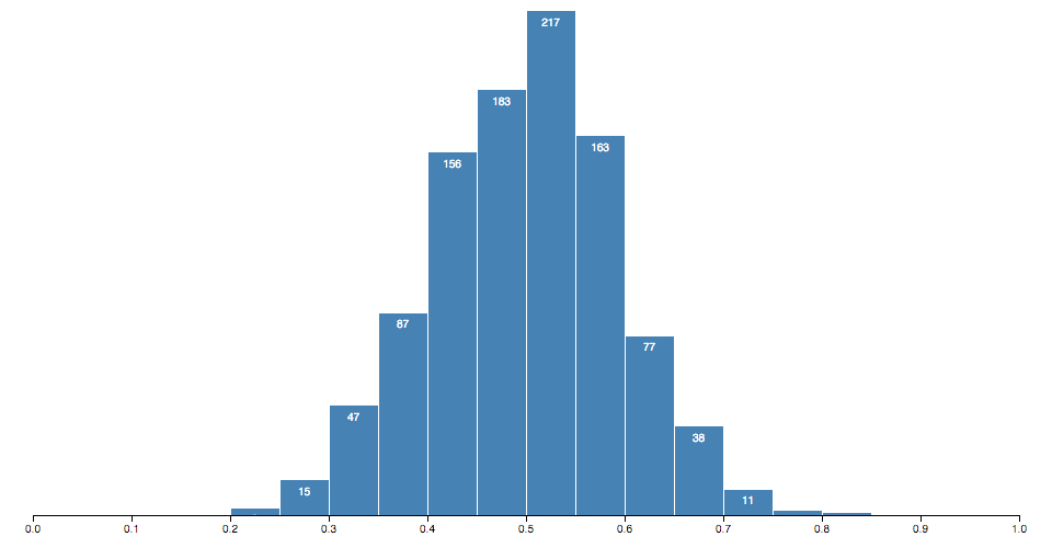 Binning groups discrete samples into a smaller number of consecutive, non-overlapping intervals.
They are often used to visualize the distribution of numerical data as histograms.
# d3.bin() · Source, Examples
Constructs a new bin generator with the default settings.
# bin(data) · Source, Examples
Bins the given iterable of data samples.
Returns an array of bins, where each bin is an array containing the associated elements from the input data.
Thus, the
Binning groups discrete samples into a smaller number of consecutive, non-overlapping intervals.
They are often used to visualize the distribution of numerical data as histograms.
# d3.bin() · Source, Examples
Constructs a new bin generator with the default settings.
# bin(data) · Source, Examples
Bins the given iterable of data samples.
Returns an array of bins, where each bin is an array containing the associated elements from the input data.
Thus, the length of the bin is the number of elements in that bin.
Each bin has two additional attributes:
x0 - the lower bound of the bin (inclusive).
x1 - the upper bound of the bin (exclusive, except for the last bin).
# bin.value([value]) · Source, Examples
If value is specified, sets the value accessor to the specified function or constant and returns this bin generator.
If value is not specified, returns the current value accessor, which defaults to the identity function.
When bins are generated, the value accessor will be invoked for each element in the input data array, being passed the element d, the index i, and the array data as three arguments.
The default value accessor assumes that the input data are orderable (comparable), such as numbers or dates.
If your data are not, then you should specify an accessor that returns the corresponding orderable value for a given datum.
This is similar to mapping your data to values before invoking the bin generator, but has the benefit that the input data remains associated with the returned bins, thereby making it easier to access other fields of the data.
# bin.domain([domain]) · Source, Examples
If domain is specified, sets the domain accessor to the specified function or array and returns this bin generator.
If domain is not specified, returns the current domain accessor, which defaults to extent.
The bin domain is defined as an array [min, max], where min is the minimum observable value and max is the maximum observable value; both values are inclusive.
Any value outside of this domain will be ignored when the bins are generated.
For example, if you are using the bin generator in conjunction with a linear scale x, you might say:
var bin = d3.bin()
.domain(x.domain())
.thresholds(x.ticks(20));
You can then compute the bins from an array of numbers like so:
var bins = bin(numbers);
If the default extent domain is used and the thresholds are specified as a count (rather than explicit values), then the computed domain will be niced such that all bins are uniform width.
Note that the domain accessor is invoked on the materialized array of values, not on the input data array.
# bin.thresholds([count]) · Source, Examples
# bin.thresholds([thresholds])
If thresholds is specified, sets the threshold generator to the specified function or array and returns this bin generator.
If thresholds is not specified, returns the current threshold generator, which by default implements Sturges’ formula.
(Thus by default, the values to be binned must be numbers!) Thresholds are defined as an array of values [x0, x1, …].
Any value less than x0 will be placed in the first bin; any value greater than or equal to x0 but less than x1 will be placed in the second bin; and so on.
Thus, the generated bins will have thresholds.length + 1 bins.
See bin thresholds for more information.
Any threshold values outside the domain are ignored.
The first bin.x0 is always equal to the minimum domain value, and the last bin.x1 is always equal to the maximum domain value.
If a count is specified instead of an array of thresholds, then the domain will be uniformly divided into approximately count bins; see ticks.
Bin Thresholds
These functions are typically not used directly; instead, pass them to bin.thresholds.
# d3.thresholdFreedmanDiaconis(values, min, max) · Source, Examples
Returns the number of bins according to the Freedman–Diaconis rule; the input values must be numbers.
# d3.thresholdScott(values, min, max) · Source, Examples
Returns the number of bins according to Scott’s normal reference rule; the input values must be numbers.
# d3.thresholdSturges(values) · Source, Examples
Returns the number of bins according to Sturges’ formula; the input values must be numbers.
You may also implement your own threshold generator taking three arguments: the array of input values derived from the data, and the observable domain represented as min and max.
The generator may then return either the array of numeric thresholds or the count of bins; in the latter case the domain is divided uniformly into approximately count bins; see ticks.
For instance, when binning date values, you might want to use the ticks from a time scale (Example).
d3-axis
The axis component renders human-readable reference marks for scales.
This alleviates one of the more tedious tasks in visualizing data.
Installing
If you use NPM, npm install d3-axis.
Otherwise, download the latest release.
You can also load directly from d3js.org, either as a standalone library or as part of D3.
(To be useful, you’ll also want to use d3-scale and d3-selection, but these are soft dependencies.) AMD, CommonJS, and vanilla environments are supported.
In vanilla, a d3 global is exported:
<script src="https://d3js.org/d3-axis.v2.min.js"></script>
<script>
var axis = d3.axisLeft(scale);
</script>
Try d3-axis in your browser.
API Reference
Regardless of orientation, axes are always rendered at the origin.
To change the position of the axis with respect to the chart, specify a transform attribute on the containing element.
For example:
d3.select("body").append("svg")
.attr("width", 1440)
.attr("height", 30)
.append("g")
.attr("transform", "translate(0,30)")
.call(axis);
The elements created by the axis are considered part of its public API.
You can apply external stylesheets or modify the generated axis elements to customize the axis appearance.
 An axis consists of a path element of class “domain” representing the extent of the scale’s domain, followed by transformed g elements of class “tick” representing each of the scale’s ticks.
Each tick has a line element to draw the tick line, and a text element for the tick label.
For example, here is a typical bottom-oriented axis:
<g fill="none" font-size="10" font-family="sans-serif" text-anchor="middle">
<path class="domain" stroke="currentColor" d="M0.5,6V0.5H880.5V6"></path>
<g class="tick" opacity="1" transform="translate(0.5,0)">
<line stroke="currentColor" y2="6"></line>
<text fill="currentColor" y="9" dy="0.71em">0.0</text>
</g>
<g class="tick" opacity="1" transform="translate(176.5,0)">
<line stroke="currentColor" y2="6"></line>
<text fill="currentColor" y="9" dy="0.71em">0.2</text>
</g>
<g class="tick" opacity="1" transform="translate(352.5,0)">
<line stroke="currentColor" y2="6"></line>
<text fill="currentColor" y="9" dy="0.71em">0.4</text>
</g>
<g class="tick" opacity="1" transform="translate(528.5,0)">
<line stroke="currentColor" y2="6"></line>
<text fill="currentColor" y="9" dy="0.71em">0.6</text>
</g>
<g class="tick" opacity="1" transform="translate(704.5,0)">
<line stroke="currentColor" y2="6"></line>
<text fill="currentColor" y="9" dy="0.71em">0.8</text>
</g>
<g class="tick" opacity="1" transform="translate(880.5,0)">
<line stroke="currentColor" y2="6"></line>
<text fill="currentColor" y="9" dy="0.71em">1.0</text>
</g>
</g>
The orientation of an axis is fixed; to change the orientation, remove the old axis and create a new axis.
# d3.axisTop(scale) · Source
Constructs a new top-oriented axis generator for the given scale, with empty tick arguments, a tick size of 6 and padding of 3.
In this orientation, ticks are drawn above the horizontal domain path.
# d3.axisRight(scale) · Source
Constructs a new right-oriented axis generator for the given scale, with empty tick arguments, a tick size of 6 and padding of 3.
In this orientation, ticks are drawn to the right of the vertical domain path.
# d3.axisBottom(scale) · Source
Constructs a new bottom-oriented axis generator for the given scale, with empty tick arguments, a tick size of 6 and padding of 3.
In this orientation, ticks are drawn below the horizontal domain path.
# d3.axisLeft(scale) · Source
Constructs a new left-oriented axis generator for the given scale, with empty tick arguments, a tick size of 6 and padding of 3.
In this orientation, ticks are drawn to the left of the vertical domain path.
# axis(context) · Source
Render the axis to the given context, which may be either a selection of SVG containers (either SVG or G elements) or a corresponding transition.
# axis.scale([scale]) · Source
If scale is specified, sets the scale and returns the axis.
If scale is not specified, returns the current scale.
# axis.ticks(arguments…) · Source
An axis consists of a path element of class “domain” representing the extent of the scale’s domain, followed by transformed g elements of class “tick” representing each of the scale’s ticks.
Each tick has a line element to draw the tick line, and a text element for the tick label.
For example, here is a typical bottom-oriented axis:
<g fill="none" font-size="10" font-family="sans-serif" text-anchor="middle">
<path class="domain" stroke="currentColor" d="M0.5,6V0.5H880.5V6"></path>
<g class="tick" opacity="1" transform="translate(0.5,0)">
<line stroke="currentColor" y2="6"></line>
<text fill="currentColor" y="9" dy="0.71em">0.0</text>
</g>
<g class="tick" opacity="1" transform="translate(176.5,0)">
<line stroke="currentColor" y2="6"></line>
<text fill="currentColor" y="9" dy="0.71em">0.2</text>
</g>
<g class="tick" opacity="1" transform="translate(352.5,0)">
<line stroke="currentColor" y2="6"></line>
<text fill="currentColor" y="9" dy="0.71em">0.4</text>
</g>
<g class="tick" opacity="1" transform="translate(528.5,0)">
<line stroke="currentColor" y2="6"></line>
<text fill="currentColor" y="9" dy="0.71em">0.6</text>
</g>
<g class="tick" opacity="1" transform="translate(704.5,0)">
<line stroke="currentColor" y2="6"></line>
<text fill="currentColor" y="9" dy="0.71em">0.8</text>
</g>
<g class="tick" opacity="1" transform="translate(880.5,0)">
<line stroke="currentColor" y2="6"></line>
<text fill="currentColor" y="9" dy="0.71em">1.0</text>
</g>
</g>
The orientation of an axis is fixed; to change the orientation, remove the old axis and create a new axis.
# d3.axisTop(scale) · Source
Constructs a new top-oriented axis generator for the given scale, with empty tick arguments, a tick size of 6 and padding of 3.
In this orientation, ticks are drawn above the horizontal domain path.
# d3.axisRight(scale) · Source
Constructs a new right-oriented axis generator for the given scale, with empty tick arguments, a tick size of 6 and padding of 3.
In this orientation, ticks are drawn to the right of the vertical domain path.
# d3.axisBottom(scale) · Source
Constructs a new bottom-oriented axis generator for the given scale, with empty tick arguments, a tick size of 6 and padding of 3.
In this orientation, ticks are drawn below the horizontal domain path.
# d3.axisLeft(scale) · Source
Constructs a new left-oriented axis generator for the given scale, with empty tick arguments, a tick size of 6 and padding of 3.
In this orientation, ticks are drawn to the left of the vertical domain path.
# axis(context) · Source
Render the axis to the given context, which may be either a selection of SVG containers (either SVG or G elements) or a corresponding transition.
# axis.scale([scale]) · Source
If scale is specified, sets the scale and returns the axis.
If scale is not specified, returns the current scale.
# axis.ticks(arguments…) · Source
# axis.ticks([count[, specifier]])
# axis.ticks([interval[, specifier]])
Sets the arguments that will be passed to scale.ticks and scale.tickFormat when the axis is rendered, and returns the axis generator.
The meaning of the arguments depends on the axis’ scale type: most commonly, the arguments are a suggested count for the number of ticks (or a time interval for time scales), and an optional format specifier to customize how the tick values are formatted.
This method has no effect if the scale does not implement scale.ticks, as with band and point scales.
To set the tick values explicitly, use axis.tickValues.
To set the tick format explicitly, use axis.tickFormat.
For example, to generate twenty ticks with SI-prefix formatting on a linear scale, say:
axis.ticks(20, "s");
To generate ticks every fifteen minutes with a time scale, say:
axis.ticks(d3.timeMinute.every(15));
This method is also a convenience function for axis.tickArguments.
For example, this:
axis.ticks(10);
Is equivalent to:
axis.tickArguments([10]);
To generate tick values directly, use scale.ticks.
# axis.tickArguments([arguments]) · Source
If arguments is specified, sets the arguments that will be passed to scale.ticks and scale.tickFormat when the axis is rendered, and returns the axis generator.
The meaning of the arguments depends on the axis’ scale type: most commonly, the arguments are a suggested count for the number of ticks (or a time interval for time scales), and an optional format specifier to customize how the tick values are formatted.
If arguments is specified, this method has no effect if the scale does not implement scale.ticks, as with band and point scales.
To set the tick values explicitly, use axis.tickValues.
To set the tick format explicitly, use axis.tickFormat.
If arguments is not specified, returns the current tick arguments, which defaults to the empty array.
For example, to generate twenty ticks with SI-prefix formatting on a linear scale, say:
axis.tickArguments([20, "s"]);
To generate ticks every fifteen minutes with a time scale, say:
axis.tickArguments([d3.timeMinute.every(15)]);
See also axis.ticks.
# axis.tickValues([values]) · Source
If a values array is specified, the specified values are used for ticks rather than using the scale’s automatic tick generator.
If values is null, clears any previously-set explicit tick values and reverts back to the scale’s tick generator.
If values is not specified, returns the current tick values, which defaults to null.
For example, to generate ticks at specific values:
var xAxis = d3.axisBottom(x)
.tickValues([1, 2, 3, 5, 8, 13, 21]);
The explicit tick values take precedent over the tick arguments set by axis.tickArguments.
However, any tick arguments will still be passed to the scale’s tickFormat function if a tick format is not also set.
# axis.tickFormat([format]) · Source
If format is specified, sets the tick format function and returns the axis.
If format is not specified, returns the current format function, which defaults to null.
A null format indicates that the scale’s default formatter should be used, which is generated by calling scale.tickFormat.
In this case, the arguments specified by axis.tickArguments are likewise passed to scale.tickFormat.
See d3-format and d3-time-format for help creating formatters.
For example, to display integers with comma-grouping for thousands:
axis.tickFormat(d3.format(",.0f"));
More commonly, a format specifier is passed to axis.ticks:
axis.ticks(10, ",f");
This has the advantage of setting the format precision automatically based on the tick interval.
# axis.tickSize([size]) · Source
If size is specified, sets the inner and outer tick size to the specified value and returns the axis.
If size is not specified, returns the current inner tick size, which defaults to 6.
# axis.tickSizeInner([size]) · Source
If size is specified, sets the inner tick size to the specified value and returns the axis.
If size is not specified, returns the current inner tick size, which defaults to 6.
The inner tick size controls the length of the tick lines, offset from the native position of the axis.
# axis.tickSizeOuter([size]) · Source
If size is specified, sets the outer tick size to the specified value and returns the axis.
If size is not specified, returns the current outer tick size, which defaults to 6.
The outer tick size controls the length of the square ends of the domain path, offset from the native position of the axis.
Thus, the “outer ticks” are not actually ticks but part of the domain path, and their position is determined by the associated scale’s domain extent.
Thus, outer ticks may overlap with the first or last inner tick.
An outer tick size of 0 suppresses the square ends of the domain path, instead producing a straight line.
# axis.tickPadding([padding]) · Source
If padding is specified, sets the padding to the specified value in pixels and returns the axis.
If padding is not specified, returns the current padding which defaults to 3 pixels.
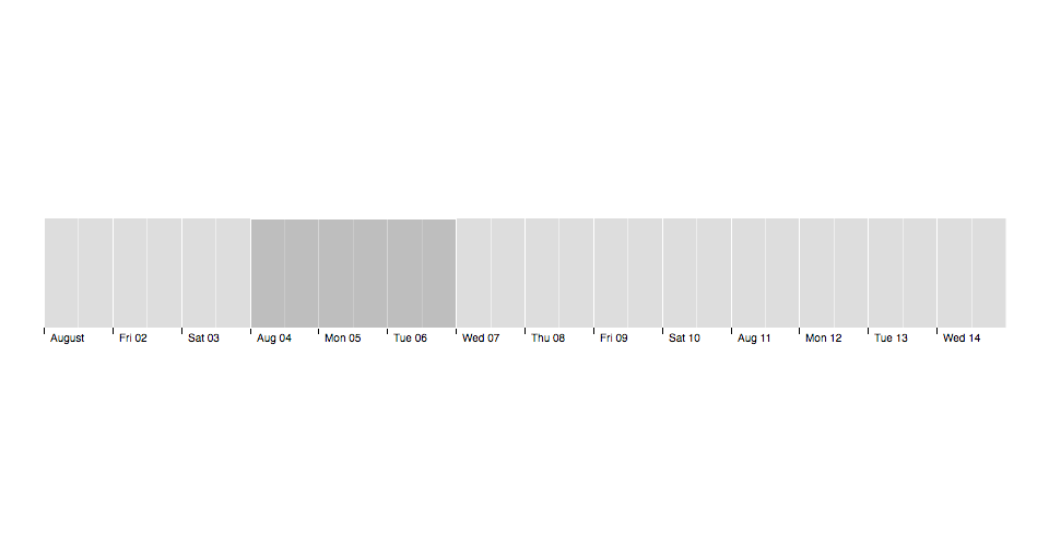
d3-brush
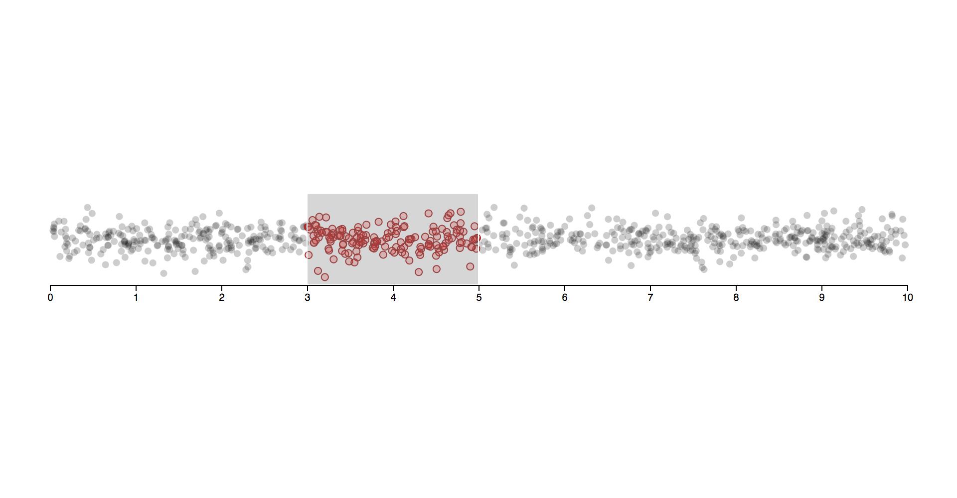
Brushing is the interactive specification a one- or two-dimensional selected region using a pointing gesture, such as by clicking and dragging the mouse.
Brushing is often used to select discrete elements, such as dots in a scatterplot or files on a desktop.
It can also be used to zoom-in to a region of interest, or to select continuous regions for cross-filtering data or live histograms:
 The d3-brush module implements brushing for mouse and touch events using SVG.
Click and drag on the brush selection to translate the selection.
Click and drag on one of the selection handles to move the corresponding edge (or edges) of the selection.
Click and drag on the invisible overlay to define a new brush selection, or click anywhere within the brushable region while holding down the META key.
Holding down the ALT key while moving the brush causes it to reposition around its center, while holding down SPACE locks the current brush size, allowing only translation.
Brushes also support programmatic control.
For example, you can listen to end events, and then initiate a transition with brush.move to snap the brush selection to semantic boundaries:
The d3-brush module implements brushing for mouse and touch events using SVG.
Click and drag on the brush selection to translate the selection.
Click and drag on one of the selection handles to move the corresponding edge (or edges) of the selection.
Click and drag on the invisible overlay to define a new brush selection, or click anywhere within the brushable region while holding down the META key.
Holding down the ALT key while moving the brush causes it to reposition around its center, while holding down SPACE locks the current brush size, allowing only translation.
Brushes also support programmatic control.
For example, you can listen to end events, and then initiate a transition with brush.move to snap the brush selection to semantic boundaries:
 Or you can have the brush recenter when you click outside the current selection:
Installing
If you use NPM, npm install d3-brush.
Otherwise, download the latest release.
You can load as a standalone library or as part of D3.
ES modules, AMD, CommonJS, and vanilla environments are supported.
In vanilla, a d3 global is exported:
<script src="https://d3js.org/d3-color.v2.min.js"></script>
<script src="https://d3js.org/d3-dispatch.v2.min.js"></script>
<script src="https://d3js.org/d3-ease.v2.min.js"></script>
<script src="https://d3js.org/d3-interpolate.v2.min.js"></script>
<script src="https://d3js.org/d3-timer.v2.min.js"></script>
<script src="https://d3js.org/d3-selection.v2.min.js"></script>
<script src="https://d3js.org/d3-transition.v2.min.js"></script>
<script src="https://d3js.org/d3-drag.v2.min.js"></script>
<script src="https://d3js.org/d3-brush.v2.min.js"></script>
<script>
var brush = d3.brush();
</script>
Try d3-brush in your browser.
API Reference
# d3.brush() · Source, Examples
Creates a new two-dimensional brush.
# d3.brushX() · Source, Examples
Creates a new one-dimensional brush along the x-dimension.
# d3.brushY() · Source
Creates a new one-dimensional brush along the y-dimension.
# brush(group) · Source, Examples
Applies the brush to the specified group, which must be a selection of SVG G elements.
This function is typically not invoked directly, and is instead invoked via selection.call.
For example, to render a brush:
svg.append("g")
.attr("class", "brush")
.call(d3.brush().on("brush", brushed));
Internally, the brush uses selection.on to bind the necessary event listeners for dragging.
The listeners use the name .brush, so you can subsequently unbind the brush event listeners as follows:
group.on(".brush", null);
The brush also creates the SVG elements necessary to display the brush selection and to receive input events for interaction.
You can add, remove or modify these elements as desired to change the brush appearance; you can also apply stylesheets to modify the brush appearance.
The structure of a two-dimensional brush is as follows:
<g class="brush" fill="none" pointer-events="all" style="-webkit-tap-highlight-color: rgba(0, 0, 0, 0);">
<rect class="overlay" pointer-events="all" cursor="crosshair" x="0" y="0" width="960" height="500"></rect>
<rect class="selection" cursor="move" fill="#777" fill-opacity="0.3" stroke="#fff" shape-rendering="crispEdges" x="112" y="194" width="182" height="83"></rect>
<rect class="handle handle--n" cursor="ns-resize" x="107" y="189" width="192" height="10"></rect>
<rect class="handle handle--e" cursor="ew-resize" x="289" y="189" width="10" height="93"></rect>
<rect class="handle handle--s" cursor="ns-resize" x="107" y="272" width="192" height="10"></rect>
<rect class="handle handle--w" cursor="ew-resize" x="107" y="189" width="10" height="93"></rect>
<rect class="handle handle--nw" cursor="nwse-resize" x="107" y="189" width="10" height="10"></rect>
<rect class="handle handle--ne" cursor="nesw-resize" x="289" y="189" width="10" height="10"></rect>
<rect class="handle handle--se" cursor="nwse-resize" x="289" y="272" width="10" height="10"></rect>
<rect class="handle handle--sw" cursor="nesw-resize" x="107" y="272" width="10" height="10"></rect>
</g>
The overlay rect covers the brushable area defined by brush.extent.
The selection rect covers the area defined by the current brush selection.
The handle rects cover the edges and corners of the brush selection, allowing the corresponding value in the brush selection to be modified interactively.
To modify the brush selection programmatically, use brush.move.
# brush.move(group, selection) · Source, Examples
Sets the active selection of the brush on the specified group, which must be a selection or a transition of SVG G elements.
The selection must be defined as an array of numbers, or null to clear the brush selection.
For a two-dimensional brush, it must be defined as [[x0, y0], [x1, y1]], where x0 is the minimum x-value, y0 is the minimum y-value, x1 is the maximum x-value, and y1 is the maximum y-value.
For an x-brush, it must be defined as [x0, x1]; for a y-brush, it must be defined as [y0, y1].
The selection may also be specified as a function which returns such an array; if a function, it is invoked for each selected element, being passed the current datum d and index i, with the this context as the current DOM element.
The returned array defines the brush selection for that element.
# brush.clear(group) · Source, Examples
An alias for brush.move with the null selection.
# brush.extent([extent]) · Source, Examples
If extent is specified, sets the brushable extent to the specified array of points [[x0, y0], [x1, y1]], where [x0, y0] is the top-left corner and [x1, y1] is the bottom-right corner, and returns this brush.
The extent may also be specified as a function which returns such an array; if a function, it is invoked for each selected element, being passed the current datum d and index i, with the this context as the current DOM element.
If extent is not specified, returns the current extent accessor, which defaults to:
function defaultExtent() {
var svg = this.ownerSVGElement || this;
if (svg.hasAttribute("viewBox")) {
svg = svg.viewBox.baseVal;
return [[svg.x, svg.y], [svg.x + svg.width, svg.y + svg.height]];
}
return [[0, 0], [svg.width.baseVal.value, svg.height.baseVal.value]];
}
This default implementation requires that the owner SVG element have a defined viewBox, or width and height attributes.
Alternatively, consider using element.getBoundingClientRect.
(In Firefox, element.clientWidth and element.clientHeight is zero for SVG elements!)
The brush extent determines the size of the invisible overlay and also constrains the brush selection; the brush selection cannot go outside the brush extent.
# brush.filter([filter]) · Source, Examples
If filter is specified, sets the filter to the specified function and returns the brush.
If filter is not specified, returns the current filter, which defaults to:
function filter(event) {
return !event.ctrlKey && !event.button;
}
If the filter returns falsey, the initiating event is ignored and no brush gesture is started.
Thus, the filter determines which input events are ignored.
The default filter ignores mousedown events on secondary buttons, since those buttons are typically intended for other purposes, such as the context menu.
# brush.touchable([touchable]) · Source
If touchable is specified, sets the touch support detector to the specified function and returns the brush.
If touchable is not specified, returns the current touch support detector, which defaults to:
function touchable() {
return navigator.maxTouchPoints || ("ontouchstart" in this);
}
Touch event listeners are only registered if the detector returns truthy for the corresponding element when the brush is applied.
The default detector works well for most browsers that are capable of touch input, but not all; Chrome’s mobile device emulator, for example, fails detection.
# brush.keyModifiers([modifiers]) · Source
If modifiers is specified, sets whether the brush listens to key events during brushing and returns the brush.
If modifiers is not specified, returns the current behavior, which defaults to true.
# brush.handleSize([size]) · Source
If size is specified, sets the size of the brush handles to the specified number and returns the brush.
If size is not specified, returns the current handle size, which defaults to six.
This method must be called before applying the brush to a selection; changing the handle size does not affect brushes that were previously rendered.
# brush.on(typenames[, listener]) · Source
If listener is specified, sets the event listener for the specified typenames and returns the brush.
If an event listener was already registered for the same type and name, the existing listener is removed before the new listener is added.
If listener is null, removes the current event listeners for the specified typenames, if any.
If listener is not specified, returns the first currently-assigned listener matching the specified typenames, if any.
When a specified event is dispatched, each listener will be invoked with the same context and arguments as selection.on listeners: the current event event and datum d, with the this context as the current DOM element.
The typenames is a string containing one or more typename separated by whitespace.
Each typename is a type, optionally followed by a period (.) and a name, such as brush.foo and brush.bar; the name allows multiple listeners to be registered for the same type.
The type must be one of the following:
start - at the start of a brush gesture, such as on mousedown.
brush - when the brush moves, such as on mousemove.
end - at the end of a brush gesture, such as on mouseup.
See dispatch.on and Brush Events for more.
# d3.brushSelection(node) · Source, Examples
Returns the current brush selection for the specified node.
Internally, an element’s brush state is stored as element.__brush; however, you should use this method rather than accessing it directly.
If the given node has no selection, returns null.
Otherwise, the selection is defined as an array of numbers.
For a two-dimensional brush, it is [[x0, y0], [x1, y1]], where x0 is the minimum x-value, y0 is the minimum y-value, x1 is the maximum x-value, and y1 is the maximum y-value.
For an x-brush, it is [x0, x1]; for a y-brush, it is [y0, y1].
Brush Events
When a brush event listener is invoked, it receives the current brush event.
The event object exposes several fields:
target - the associated brush behavior.
type - the string “start”, “brush” or “end”; see brush.on.
selection - the current brush selection.
sourceEvent - the underlying input event, such as mousemove or touchmove.
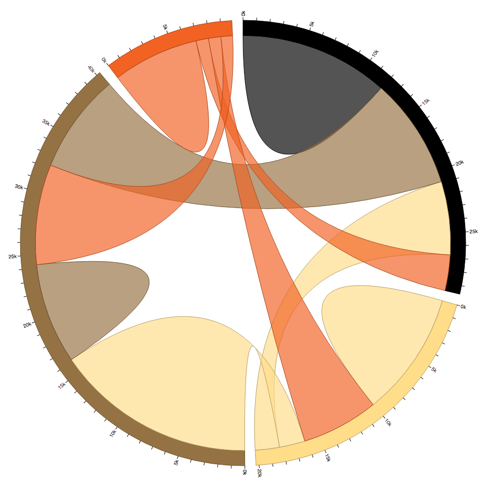
d3-chord
Visualize relationships or network flow with an aesthetically-pleasing circular layout.
Installing
If you use NPM, npm install d3-chord.
Otherwise, download the latest release.
You can also load directly from d3js.org, either as a standalone library or as part of D3.
AMD, CommonJS, and vanilla environments are supported.
In vanilla, a d3 global is exported:
<script src="https://d3js.org/d3-path.v2.min.js"></script>
<script src="https://d3js.org/d3-chord.v2.min.js"></script>
<script>
var chord = d3.chord();
</script>
API Reference
# d3.chord() <>
Constructs a new chord layout with the default settings.
# chord(matrix) <>
Computes the chord layout for the specified square matrix of size n×n, where the matrix represents the directed flow amongst a network (a complete digraph) of n nodes.
The given matrix must be an array of length n, where each element matrix[i] is an array of n numbers, where each matrix[i][j] represents the flow from the ith node in the network to the jth node.
Each number matrix[i][j] must be nonnegative, though it can be zero if there is no flow from node i to node j.
From the Circos tableviewer example:
var matrix = [
[11975, 5871, 8916, 2868],
[ 1951, 10048, 2060, 6171],
[ 8010, 16145, 8090, 8045],
[ 1013, 990, 940, 6907]
];
The return value of chord(matrix) is an array of chords, where each chord represents the combined bidirectional flow between two nodes i and j (where i may be equal to j) and is an object with the following properties:
source - the source subgroup
target - the target subgroup
Each source and target subgroup is also an object with the following properties:
startAngle - the start angle in radians
endAngle - the end angle in radians
value - the flow value matrix[i][j]
index - the node index i
The chords are typically passed to d3.ribbon to display the network relationships.
The returned array includes only chord objects for which the value matrix[i][j] or matrix[j][i] is non-zero.
Furthermore, the returned array only contains unique chords: a given chord ij represents the bidirectional flow from i to j and from j to i, and does not contain a duplicate chord ji; i and j are chosen such that the chord’s source always represents the larger of matrix[i][j] and matrix[j][i].
The chords array also defines a secondary array of length n, chords.groups, where each group represents the combined outflow for node i, corresponding to the elements matrix[i][0 … n - 1], and is an object with the following properties:
startAngle - the start angle in radians
endAngle - the end angle in radians
value - the total outgoing flow value for node i
index - the node index i
The groups are typically passed to d3.arc to produce a donut chart around the circumference of the chord layout.
# chord.padAngle([angle]) <>
If angle is specified, sets the pad angle between adjacent groups to the specified number in radians and returns this chord layout.
If angle is not specified, returns the current pad angle, which defaults to zero.
# chord.sortGroups([compare]) <>
If compare is specified, sets the group comparator to the specified function or null and returns this chord layout.
If compare is not specified, returns the current group comparator, which defaults to null.
If the group comparator is non-null, it is used to sort the groups by their total outflow.
See also d3.ascending and d3.descending.
# chord.sortSubgroups([compare]) <>
If compare is specified, sets the subgroup comparator to the specified function or null and returns this chord layout.
If compare is not specified, returns the current subgroup comparator, which defaults to null.
If the subgroup comparator is non-null, it is used to sort the subgroups corresponding to matrix[i][0 … n - 1] for a given group i by their total outflow.
See also d3.ascending and d3.descending.
# chord.sortChords([compare]) <>
If compare is specified, sets the chord comparator to the specified function or null and returns this chord layout.
If compare is not specified, returns the current chord comparator, which defaults to null.
If the chord comparator is non-null, it is used to sort the chords by their combined flow; this only affects the z-order of the chords.
See also d3.ascending and d3.descending.
# d3.ribbon() <>
Creates a new ribbon generator with the default settings.
# ribbon(arguments…) <>
Generates a ribbon for the given arguments.
The arguments are arbitrary; they are simply propagated to the ribbon generator’s accessor functions along with the this object.
For example, with the default settings, a chord object expected:
var ribbon = d3.ribbon();
ribbon({
source: {startAngle: 0.7524114, endAngle: 1.1212972, radius: 240},
target: {startAngle: 1.8617078, endAngle: 1.9842927, radius: 240}
}); // "M164.0162810494058,-175.21032946354026A240,240,0,0,1,216.1595644740915,-104.28347273835429Q0,0,229.9158815306728,68.8381247563705A240,240,0,0,1,219.77316791012538,96.43523560788266Q0,0,164.0162810494058,-175.21032946354026Z"
Or equivalently if the radius is instead defined as a constant:
var ribbon = d3.ribbon()
.radius(240);
ribbon({
source: {startAngle: 0.7524114, endAngle: 1.1212972},
target: {startAngle: 1.8617078, endAngle: 1.9842927}
}); // "M164.0162810494058,-175.21032946354026A240,240,0,0,1,216.1595644740915,-104.28347273835429Q0,0,229.9158815306728,68.8381247563705A240,240,0,0,1,219.77316791012538,96.43523560788266Q0,0,164.0162810494058,-175.21032946354026Z"
If the ribbon generator has a context, then the ribbon is rendered to this context as a sequence of path method calls and this function returns void.
Otherwise, a path data string is returned.
# ribbon.source([source]) <>
If source is specified, sets the source accessor to the specified function and returns this ribbon generator.
If source is not specified, returns the current source accessor, which defaults to:
function source(d) {
return d.source;
}
# ribbon.target([target]) <>
If target is specified, sets the target accessor to the specified function and returns this ribbon generator.
If target is not specified, returns the current target accessor, which defaults to:
function target(d) {
return d.target;
}
# ribbon.radius([radius]) <>
If radius is specified, sets the source and target radius accessor to the specified function and returns this ribbon generator.
If radius is not specified, returns the current source radius accessor, which defaults to:
function radius(d) {
return d.radius;
}
# ribbon.sourceRadius([radius]) <>
If radius is specified, sets the source radius accessor to the specified function and returns this ribbon generator.
If radius is not specified, returns the current source radius accessor, which defaults to:
function radius(d) {
return d.radius;
}
# ribbon.targetRadius([radius]) <>
If radius is specified, sets the target radius accessor to the specified function and returns this ribbon generator.
If radius is not specified, returns the current target radius accessor, which defaults to:
function radius(d) {
return d.radius;
}
By convention, the target radius in asymmetric chord diagrams is typically inset from the source radius, resulting in a gap between the end of the directed link and its associated group arc.
# ribbon.startAngle([angle]) <>
If angle is specified, sets the start angle accessor to the specified function and returns this ribbon generator.
If angle is not specified, returns the current start angle accessor, which defaults to:
function startAngle(d) {
return d.startAngle;
}
The angle is specified in radians, with 0 at -y (12 o’clock) and positive angles proceeding clockwise.
# ribbon.endAngle([angle]) <>
If angle is specified, sets the end angle accessor to the specified function and returns this ribbon generator.
If angle is not specified, returns the current end angle accessor, which defaults to:
function endAngle(d) {
return d.endAngle;
}
The angle is specified in radians, with 0 at -y (12 o’clock) and positive angles proceeding clockwise.
# ribbon.padAngle([angle]) <>
If angle is specified, sets the pad angle accessor to the specified function and returns this ribbon generator.
If angle is not specified, returns the current pad angle accessor, which defaults to:
function padAngle() {
return 0;
}
The pad angle specifies the angular gap between adjacent ribbons.
# ribbon.context([context]) <>
If context is specified, sets the context and returns this ribbon generator.
If context is not specified, returns the current context, which defaults to null.
If the context is not null, then the generated ribbon is rendered to this context as a sequence of path method calls.
Otherwise, a path data string representing the generated ribbon is returned.
See also d3-path.
# d3.ribbonArrow() <>
Creates a new arrow ribbon generator with the default settings.
# ribbonArrow.headRadius([radius]) <>
If radius is specified, sets the arrowhead radius accessor to the specified function and returns this ribbon generator.
If radius is not specified, returns the current arrowhead radius accessor, which defaults to:
function headRadius() {
return 10;
}
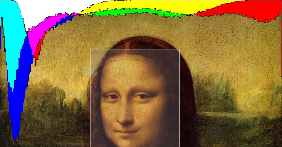
d3-color
Even though your browser understands a lot about colors, it doesn’t offer much help in manipulating colors through JavaScript.
The d3-color module therefore provides representations for various color spaces, allowing specification, conversion and manipulation.
(Also see d3-interpolate for color interpolation.)
For example, take the color named “steelblue”:
var c = d3.color("steelblue"); // {r: 70, g: 130, b: 180, opacity: 1}
Let’s try converting it to HSL:
var c = d3.hsl("steelblue"); // {h: 207.27…, s: 0.44, l: 0.4902…, opacity: 1}
Now rotate the hue by 90°, bump up the saturation, and format as a string for CSS:
c.h += 90;
c.s += 0.2;
c + ""; // rgb(198, 45, 205)
To fade the color slightly:
c.opacity = 0.8;
c + ""; // rgba(198, 45, 205, 0.8)
In addition to the ubiquitous and machine-friendly RGB and HSL color space, d3-color supports color spaces that are designed for humans:
CIELAB (a.k.a. “Lab”)
CIELChab (a.k.a. “LCh” or “HCL”)
Dave Green’s Cubehelix
Cubehelix features monotonic lightness, while CIELAB and its polar form CIELChab are perceptually uniform.
Extensions
For additional color spaces, see:
d3-cam16
d3-cam02
d3-hsv
d3-hcg
d3-hsluv
To measure color differences, see:
d3-color-difference
Installing
If you use NPM, npm install d3-color.
Otherwise, download the latest release.
You can also load directly from d3js.org, either as a standalone library or as part of D3.
AMD, CommonJS, and vanilla environments are supported.
In vanilla, a d3 global is exported:
<script src="https://d3js.org/d3-color.v2.min.js"></script>
<script>
var steelblue = d3.rgb("steelblue");
</script>
Try d3-color in your browser.
API Reference
# d3.color(specifier) <>
Parses the specified CSS Color Module Level 3 specifier string, returning an RGB or HSL color, along with CSS Color Module Level 4 hex specifier strings.
If the specifier was not valid, null is returned.
Some examples:
rgb(255, 255, 255)
rgb(10%, 20%, 30%)
rgba(255, 255, 255, 0.4)
rgba(10%, 20%, 30%, 0.4)
hsl(120, 50%, 20%)
hsla(120, 50%, 20%, 0.4)
#ffeeaa
#fea
#ffeeaa22
#fea2
steelblue
The list of supported named colors is specified by CSS.
Note: this function may also be used with instanceof to test if an object is a color instance.
The same is true of color subclasses, allowing you to test whether a color is in a particular color space.
# color.opacity
This color’s opacity, typically in the range [0, 1].
# color.rgb() <>
Returns the RGB equivalent of this color.
For RGB colors, that’s this.
# color.copy([values]) <>
Returns a copy of this color.
If values is specified, any enumerable own properties of values are assigned to the new returned color.
For example, to derive a copy of a color with opacity 0.5, say
color.copy({opacity: 0.5})
# color.brighter([k]) <>
Returns a brighter copy of this color.
If k is specified, it controls how much brighter the returned color should be.
If k is not specified, it defaults to 1.
The behavior of this method is dependent on the implementing color space.
# color.darker([k]) <>
Returns a darker copy of this color.
If k is specified, it controls how much darker the returned color should be.
If k is not specified, it defaults to 1.
The behavior of this method is dependent on the implementing color space.
# color.displayable() <>
Returns true if and only if the color is displayable on standard hardware.
For example, this returns false for an RGB color if any channel value is less than zero or greater than 255 when rounded, or if the opacity is not in the range [0, 1].
# color.formatHex() <>
Returns a hexadecimal string representing this color in RGB space, such as #f7eaba.
If this color is not displayable, a suitable displayable color is returned instead.
For example, RGB channel values greater than 255 are clamped to 255.
# color.formatHsl() <>
Returns a string representing this color according to the CSS Color Module Level 3 specification, such as hsl(257, 50%, 80%) or hsla(257, 50%, 80%, 0.2).
If this color is not displayable, a suitable displayable color is returned instead by clamping S and L channel values to the interval [0, 100].
# color.formatRgb() <>
Returns a string representing this color according to the CSS Object Model specification, such as rgb(247, 234, 186) or rgba(247, 234, 186, 0.2).
If this color is not displayable, a suitable displayable color is returned instead by clamping RGB channel values to the interval [0, 255].
# color.toString() <>
An alias for color.formatRgb.
# d3.rgb(r, g, b[, opacity]) <>
# d3.rgb(specifier)
# d3.rgb(color)
Constructs a new RGB color.
The channel values are exposed as r, g and b properties on the returned instance.
Use the RGB color picker to explore this color space.
If r, g and b are specified, these represent the channel values of the returned color; an opacity may also be specified.
If a CSS Color Module Level 3 specifier string is specified, it is parsed and then converted to the RGB color space.
See color for examples.
If a color instance is specified, it is converted to the RGB color space using color.rgb.
Note that unlike color.rgb this method always returns a new instance, even if color is already an RGB color.
# d3.hsl(h, s, l[, opacity]) <>
# d3.hsl(specifier)
# d3.hsl(color)
Constructs a new HSL color.
The channel values are exposed as h, s and l properties on the returned instance.
Use the HSL color picker to explore this color space.
If h, s and l are specified, these represent the channel values of the returned color; an opacity may also be specified.
If a CSS Color Module Level 3 specifier string is specified, it is parsed and then converted to the HSL color space.
See color for examples.
If a color instance is specified, it is converted to the RGB color space using color.rgb and then converted to HSL.
(Colors already in the HSL color space skip the conversion to RGB.)
# d3.lab(l, a, b[, opacity]) <>
# d3.lab(specifier)
# d3.lab(color)
Constructs a new CIELAB color.
The channel values are exposed as l, a and b properties on the returned instance.
Use the CIELAB color picker to explore this color space.
The value of l is typically in the range [0, 100], while a and b are typically in [-160, +160].
If l, a and b are specified, these represent the channel values of the returned color; an opacity may also be specified.
If a CSS Color Module Level 3 specifier string is specified, it is parsed and then converted to the CIELAB color space.
See color for examples.
If a color instance is specified, it is converted to the RGB color space using color.rgb and then converted to CIELAB.
(Colors already in the CIELAB color space skip the conversion to RGB, and colors in the HCL color space are converted directly to CIELAB.)
# d3.gray(l[, opacity]) <>
Constructs a new CIELAB color with the specified l value and a = b = 0.
# d3.hcl(h, c, l[, opacity]) <>
# d3.hcl(specifier)
# d3.hcl(color)
Equivalent to d3.lch, but with reversed argument order.
# d3.lch(l, c, h[, opacity]) <>
# d3.lch(specifier)
# d3.lch(color)
Constructs a new CIELChab color.
The channel values are exposed as l, c and h properties on the returned instance.
Use the CIELChab color picker to explore this color space.
The value of l is typically in the range [0, 100], c is typically in [0, 230], and h is typically in [0, 360).
If l, c, and h are specified, these represent the channel values of the returned color; an opacity may also be specified.
If a CSS Color Module Level 3 specifier string is specified, it is parsed and then converted to CIELChab color space.
See color for examples.
If a color instance is specified, it is converted to the RGB color space using color.rgb and then converted to CIELChab.
(Colors already in CIELChab color space skip the conversion to RGB, and colors in CIELAB color space are converted directly to CIELChab.)
# d3.cubehelix(h, s, l[, opacity]) <>
# d3.cubehelix(specifier)
# d3.cubehelix(color)
Constructs a new Cubehelix color.
The channel values are exposed as h, s and l properties on the returned instance.
Use the Cubehelix color picker to explore this color space.
If h, s and l are specified, these represent the channel values of the returned color; an opacity may also be specified.
If a CSS Color Module Level 3 specifier string is specified, it is parsed and then converted to the Cubehelix color space.
See color for examples.
If a color instance is specified, it is converted to the RGB color space using color.rgb and then converted to Cubehelix.
(Colors already in the Cubehelix color space skip the conversion to RGB.)
d3-scale-chromatic
This module provides sequential, diverging and categorical color schemes designed to work with d3-scale’s d3.scaleOrdinal and d3.scaleSequential.
Most of these schemes are derived from Cynthia A.
Brewer’s ColorBrewer.
Since ColorBrewer publishes only discrete color schemes, the sequential and diverging scales are interpolated using uniform B-splines.
For example, to create a categorical color scale using the Accent color scheme:
var accent = d3.scaleOrdinal(d3.schemeAccent);
To create a sequential discrete nine-color scale using the Blues color scheme:
var blues = d3.scaleOrdinal(d3.schemeBlues[9]);
To create a diverging, continuous color scale using the PiYG color scheme:
var piyg = d3.scaleSequential(d3.interpolatePiYG);
Installing
If you use NPM, npm install d3-scale-chromatic.
Otherwise, download the latest release or load directly from d3js.org as a standalone library.
AMD, CommonJS, and vanilla environments are supported.
In vanilla, a d3 global is exported:
<script src="https://d3js.org/d3-color.v2.min.js"></script>
<script src="https://d3js.org/d3-interpolate.v2.min.js"></script>
<script src="https://d3js.org/d3-scale-chromatic.v2.min.js"></script>
<script>
var yellow = d3.interpolateYlGn(0), // "rgb(255, 255, 229)"
yellowGreen = d3.interpolateYlGn(0.5), // "rgb(120, 197, 120)"
green = d3.interpolateYlGn(1); // "rgb(0, 69, 41)"
</script>
Or, as part of the D3 default bundle:
<script src="https://d3js.org/d3.v6.min.js"></script>
<script>
var yellow = d3.interpolateYlGn(0), // "rgb(255, 255, 229)"
yellowGreen = d3.interpolateYlGn(0.5), // "rgb(120, 197, 120)"
green = d3.interpolateYlGn(1); // "rgb(0, 69, 41)"
</script>
Try d3-scale-chromatic in your browser.
API Reference
Categorical
# d3.schemeCategory10 <>
 An array of ten categorical colors represented as RGB hexadecimal strings.
# d3.schemeAccent <>
An array of ten categorical colors represented as RGB hexadecimal strings.
# d3.schemeAccent <>
 An array of eight categorical colors represented as RGB hexadecimal strings.
# d3.schemeDark2 <>
An array of eight categorical colors represented as RGB hexadecimal strings.
# d3.schemeDark2 <>
 An array of eight categorical colors represented as RGB hexadecimal strings.
# d3.schemePaired <>
An array of eight categorical colors represented as RGB hexadecimal strings.
# d3.schemePaired <>
 An array of twelve categorical colors represented as RGB hexadecimal strings.
# d3.schemePastel1 <>
An array of twelve categorical colors represented as RGB hexadecimal strings.
# d3.schemePastel1 <>
 An array of nine categorical colors represented as RGB hexadecimal strings.
# d3.schemePastel2 <>
An array of nine categorical colors represented as RGB hexadecimal strings.
# d3.schemePastel2 <>
 An array of eight categorical colors represented as RGB hexadecimal strings.
# d3.schemeSet1 <>
An array of eight categorical colors represented as RGB hexadecimal strings.
# d3.schemeSet1 <>
 An array of nine categorical colors represented as RGB hexadecimal strings.
# d3.schemeSet2 <>
An array of nine categorical colors represented as RGB hexadecimal strings.
# d3.schemeSet2 <>
 An array of eight categorical colors represented as RGB hexadecimal strings.
# d3.schemeSet3 <>
An array of eight categorical colors represented as RGB hexadecimal strings.
# d3.schemeSet3 <>
 An array of twelve categorical colors represented as RGB hexadecimal strings.
# d3.schemeTableau10 <>
An array of twelve categorical colors represented as RGB hexadecimal strings.
# d3.schemeTableau10 <>
 An array of ten categorical colors authored by Tableau as part of Tableau 10 represented as RGB hexadecimal strings.
Diverging
Diverging color schemes are available as continuous interpolators (often used with d3.scaleSequential) and as discrete schemes (often used with d3.scaleOrdinal).
Each discrete scheme, such as d3.schemeBrBG, is represented as an array of arrays of hexadecimal color strings.
The kth element of this array contains the color scheme of size k; for example, d3.schemeBrBG[9] contains an array of nine strings representing the nine colors of the brown-blue-green diverging color scheme.
Diverging color schemes support a size k ranging from 3 to 11.
# d3.interpolateBrBG(t) <>
# d3.schemeBrBG[k]
 Given a number t in the range [0,1], returns the corresponding color from the “BrBG” diverging color scheme represented as an RGB string.
# d3.interpolatePRGn(t) <>
Given a number t in the range [0,1], returns the corresponding color from the “BrBG” diverging color scheme represented as an RGB string.
# d3.interpolatePRGn(t) <>
# d3.schemePRGn[k]
 Given a number t in the range [0,1], returns the corresponding color from the “PRGn” diverging color scheme represented as an RGB string.
# d3.interpolatePiYG(t) <>
Given a number t in the range [0,1], returns the corresponding color from the “PRGn” diverging color scheme represented as an RGB string.
# d3.interpolatePiYG(t) <>
# d3.schemePiYG[k]
 Given a number t in the range [0,1], returns the corresponding color from the “PiYG” diverging color scheme represented as an RGB string.
# d3.interpolatePuOr(t) <>
Given a number t in the range [0,1], returns the corresponding color from the “PiYG” diverging color scheme represented as an RGB string.
# d3.interpolatePuOr(t) <>
# d3.schemePuOr[k]
 Given a number t in the range [0,1], returns the corresponding color from the “PuOr” diverging color scheme represented as an RGB string.
# d3.interpolateRdBu(t) <>
Given a number t in the range [0,1], returns the corresponding color from the “PuOr” diverging color scheme represented as an RGB string.
# d3.interpolateRdBu(t) <>
# d3.schemeRdBu[k]
 Given a number t in the range [0,1], returns the corresponding color from the “RdBu” diverging color scheme represented as an RGB string.
# d3.interpolateRdGy(t) <>
Given a number t in the range [0,1], returns the corresponding color from the “RdBu” diverging color scheme represented as an RGB string.
# d3.interpolateRdGy(t) <>
# d3.schemeRdGy[k]
 Given a number t in the range [0,1], returns the corresponding color from the “RdGy” diverging color scheme represented as an RGB string.
# d3.interpolateRdYlBu(t) <>
Given a number t in the range [0,1], returns the corresponding color from the “RdGy” diverging color scheme represented as an RGB string.
# d3.interpolateRdYlBu(t) <>
# d3.schemeRdYlBu[k]
 Given a number t in the range [0,1], returns the corresponding color from the “RdYlBu” diverging color scheme represented as an RGB string.
# d3.interpolateRdYlGn(t) <>
Given a number t in the range [0,1], returns the corresponding color from the “RdYlBu” diverging color scheme represented as an RGB string.
# d3.interpolateRdYlGn(t) <>
# d3.schemeRdYlGn[k]
 Given a number t in the range [0,1], returns the corresponding color from the “RdYlGn” diverging color scheme represented as an RGB string.
# d3.interpolateSpectral(t) <>
Given a number t in the range [0,1], returns the corresponding color from the “RdYlGn” diverging color scheme represented as an RGB string.
# d3.interpolateSpectral(t) <>
# d3.schemeSpectral[k]
 Given a number t in the range [0,1], returns the corresponding color from the “Spectral” diverging color scheme represented as an RGB string.
Sequential (Single Hue)
Sequential, single-hue color schemes are available as continuous interpolators (often used with d3.scaleSequential) and as discrete schemes (often used with d3.scaleOrdinal).
Each discrete scheme, such as d3.schemeBlues, is represented as an array of arrays of hexadecimal color strings.
The kth element of this array contains the color scheme of size k; for example, d3.schemeBlues[9] contains an array of nine strings representing the nine colors of the blue sequential color scheme.
Sequential, single-hue color schemes support a size k ranging from 3 to 9.
# d3.interpolateBlues(t) <>
# d3.schemeBlues[k]
 Given a number t in the range [0,1], returns the corresponding color from the “Blues” sequential color scheme represented as an RGB string.
# d3.interpolateGreens(t) <>
Given a number t in the range [0,1], returns the corresponding color from the “Blues” sequential color scheme represented as an RGB string.
# d3.interpolateGreens(t) <>
# d3.schemeGreens[k]
 Given a number t in the range [0,1], returns the corresponding color from the “Greens” sequential color scheme represented as an RGB string.
# d3.interpolateGreys(t) <>
Given a number t in the range [0,1], returns the corresponding color from the “Greens” sequential color scheme represented as an RGB string.
# d3.interpolateGreys(t) <>
# d3.schemeGreys[k]
 Given a number t in the range [0,1], returns the corresponding color from the “Greys” sequential color scheme represented as an RGB string.
# d3.interpolateOranges(t) <>
Given a number t in the range [0,1], returns the corresponding color from the “Greys” sequential color scheme represented as an RGB string.
# d3.interpolateOranges(t) <>
# d3.schemeOranges[k]
 Given a number t in the range [0,1], returns the corresponding color from the “Oranges” sequential color scheme represented as an RGB string.
# d3.interpolatePurples(t) <>
Given a number t in the range [0,1], returns the corresponding color from the “Oranges” sequential color scheme represented as an RGB string.
# d3.interpolatePurples(t) <>
# d3.schemePurples[k]
 Given a number t in the range [0,1], returns the corresponding color from the “Purples” sequential color scheme represented as an RGB string.
# d3.interpolateReds(t) <>
Given a number t in the range [0,1], returns the corresponding color from the “Purples” sequential color scheme represented as an RGB string.
# d3.interpolateReds(t) <>
# d3.schemeReds[k]
 Given a number t in the range [0,1], returns the corresponding color from the “Reds” sequential color scheme represented as an RGB string.
Sequential (Multi-Hue)
Sequential, multi-hue color schemes are available as continuous interpolators (often used with d3.scaleSequential) and as discrete schemes (often used with d3.scaleOrdinal).
Each discrete scheme, such as d3.schemeBuGn, is represented as an array of arrays of hexadecimal color strings.
The kth element of this array contains the color scheme of size k; for example, d3.schemeBuGn[9] contains an array of nine strings representing the nine colors of the blue-green sequential color scheme.
Sequential, multi-hue color schemes support a size k ranging from 3 to 9.
# d3.interpolateTurbo(t) <>
 Given a number t in the range [0,1], returns the corresponding color from the “turbo” color scheme by Anton Mikhailov.
# d3.interpolateViridis(t) <>
Given a number t in the range [0,1], returns the corresponding color from the “turbo” color scheme by Anton Mikhailov.
# d3.interpolateViridis(t) <>
 Given a number t in the range [0,1], returns the corresponding color from the “viridis” perceptually-uniform color scheme designed by van der Walt, Smith and Firing for matplotlib, represented as an RGB string.
# d3.interpolateInferno(t) <>
Given a number t in the range [0,1], returns the corresponding color from the “viridis” perceptually-uniform color scheme designed by van der Walt, Smith and Firing for matplotlib, represented as an RGB string.
# d3.interpolateInferno(t) <>
 Given a number t in the range [0,1], returns the corresponding color from the “inferno” perceptually-uniform color scheme designed by van der Walt and Smith for matplotlib, represented as an RGB string.
# d3.interpolateMagma(t) <>
Given a number t in the range [0,1], returns the corresponding color from the “inferno” perceptually-uniform color scheme designed by van der Walt and Smith for matplotlib, represented as an RGB string.
# d3.interpolateMagma(t) <>
 Given a number t in the range [0,1], returns the corresponding color from the “magma” perceptually-uniform color scheme designed by van der Walt and Smith for matplotlib, represented as an RGB string.
# d3.interpolatePlasma(t) <>
Given a number t in the range [0,1], returns the corresponding color from the “magma” perceptually-uniform color scheme designed by van der Walt and Smith for matplotlib, represented as an RGB string.
# d3.interpolatePlasma(t) <>
 Given a number t in the range [0,1], returns the corresponding color from the “plasma” perceptually-uniform color scheme designed by van der Walt and Smith for matplotlib, represented as an RGB string.
# d3.interpolateCividis(t) <>
Given a number t in the range [0,1], returns the corresponding color from the “plasma” perceptually-uniform color scheme designed by van der Walt and Smith for matplotlib, represented as an RGB string.
# d3.interpolateCividis(t) <>
 Given a number t in the range [0,1], returns the corresponding color from the “cividis” color vision deficiency-optimized color scheme designed by Nuñez, Anderton, and Renslow, represented as an RGB string.
# d3.interpolateWarm(t) <>
Given a number t in the range [0,1], returns the corresponding color from the “cividis” color vision deficiency-optimized color scheme designed by Nuñez, Anderton, and Renslow, represented as an RGB string.
# d3.interpolateWarm(t) <>
 Given a number t in the range [0,1], returns the corresponding color from a 180° rotation of Niccoli’s perceptual rainbow, represented as an RGB string.
# d3.interpolateCool(t) <>
Given a number t in the range [0,1], returns the corresponding color from a 180° rotation of Niccoli’s perceptual rainbow, represented as an RGB string.
# d3.interpolateCool(t) <>
 Given a number t in the range [0,1], returns the corresponding color from Niccoli’s perceptual rainbow, represented as an RGB string.
# d3.interpolateCubehelixDefault(t) <>
Given a number t in the range [0,1], returns the corresponding color from Niccoli’s perceptual rainbow, represented as an RGB string.
# d3.interpolateCubehelixDefault(t) <>
 Given a number t in the range [0,1], returns the corresponding color from Green’s default Cubehelix represented as an RGB string.
# d3.interpolateBuGn(t) <>
Given a number t in the range [0,1], returns the corresponding color from Green’s default Cubehelix represented as an RGB string.
# d3.interpolateBuGn(t) <>
# d3.schemeBuGn[k]
 Given a number t in the range [0,1], returns the corresponding color from the “BuGn” sequential color scheme represented as an RGB string.
# d3.interpolateBuPu(t) <>
Given a number t in the range [0,1], returns the corresponding color from the “BuGn” sequential color scheme represented as an RGB string.
# d3.interpolateBuPu(t) <>
# d3.schemeBuPu[k]
 Given a number t in the range [0,1], returns the corresponding color from the “BuPu” sequential color scheme represented as an RGB string.
# d3.interpolateGnBu(t) <>
Given a number t in the range [0,1], returns the corresponding color from the “BuPu” sequential color scheme represented as an RGB string.
# d3.interpolateGnBu(t) <>
# d3.schemeGnBu[k]
 Given a number t in the range [0,1], returns the corresponding color from the “GnBu” sequential color scheme represented as an RGB string.
# d3.interpolateOrRd(t) <>
Given a number t in the range [0,1], returns the corresponding color from the “GnBu” sequential color scheme represented as an RGB string.
# d3.interpolateOrRd(t) <>
# d3.schemeOrRd[k]
 Given a number t in the range [0,1], returns the corresponding color from the “OrRd” sequential color scheme represented as an RGB string.
# d3.interpolatePuBuGn(t) <>
Given a number t in the range [0,1], returns the corresponding color from the “OrRd” sequential color scheme represented as an RGB string.
# d3.interpolatePuBuGn(t) <>
# d3.schemePuBuGn[k]
 Given a number t in the range [0,1], returns the corresponding color from the “PuBuGn” sequential color scheme represented as an RGB string.
# d3.interpolatePuBu(t) <>
Given a number t in the range [0,1], returns the corresponding color from the “PuBuGn” sequential color scheme represented as an RGB string.
# d3.interpolatePuBu(t) <>
# d3.schemePuBu[k]
 Given a number t in the range [0,1], returns the corresponding color from the “PuBu” sequential color scheme represented as an RGB string.
# d3.interpolatePuRd(t) <>
Given a number t in the range [0,1], returns the corresponding color from the “PuBu” sequential color scheme represented as an RGB string.
# d3.interpolatePuRd(t) <>
# d3.schemePuRd[k]
 Given a number t in the range [0,1], returns the corresponding color from the “PuRd” sequential color scheme represented as an RGB string.
# d3.interpolateRdPu(t) <>
Given a number t in the range [0,1], returns the corresponding color from the “PuRd” sequential color scheme represented as an RGB string.
# d3.interpolateRdPu(t) <>
# d3.schemeRdPu[k]
 Given a number t in the range [0,1], returns the corresponding color from the “RdPu” sequential color scheme represented as an RGB string.
# d3.interpolateYlGnBu(t) <>
Given a number t in the range [0,1], returns the corresponding color from the “RdPu” sequential color scheme represented as an RGB string.
# d3.interpolateYlGnBu(t) <>
# d3.schemeYlGnBu[k]
 Given a number t in the range [0,1], returns the corresponding color from the “YlGnBu” sequential color scheme represented as an RGB string.
# d3.interpolateYlGn(t) <>
Given a number t in the range [0,1], returns the corresponding color from the “YlGnBu” sequential color scheme represented as an RGB string.
# d3.interpolateYlGn(t) <>
# d3.schemeYlGn[k]
 Given a number t in the range [0,1], returns the corresponding color from the “YlGn” sequential color scheme represented as an RGB string.
# d3.interpolateYlOrBr(t) <>
Given a number t in the range [0,1], returns the corresponding color from the “YlGn” sequential color scheme represented as an RGB string.
# d3.interpolateYlOrBr(t) <>
# d3.schemeYlOrBr[k]
 Given a number t in the range [0,1], returns the corresponding color from the “YlOrBr” sequential color scheme represented as an RGB string.
# d3.interpolateYlOrRd(t) <>
Given a number t in the range [0,1], returns the corresponding color from the “YlOrBr” sequential color scheme represented as an RGB string.
# d3.interpolateYlOrRd(t) <>
# d3.schemeYlOrRd[k]
 Given a number t in the range [0,1], returns the corresponding color from the “YlOrRd” sequential color scheme represented as an RGB string.
Cyclical
# d3.interpolateRainbow(t) <>
 Given a number t in the range [0,1], returns the corresponding color from d3.interpolateWarm scale from [0.0, 0.5] followed by the d3.interpolateCool scale from [0.5, 1.0], thus implementing the cyclical less-angry rainbow color scheme.
# d3.interpolateSinebow(t) <>
Given a number t in the range [0,1], returns the corresponding color from d3.interpolateWarm scale from [0.0, 0.5] followed by the d3.interpolateCool scale from [0.5, 1.0], thus implementing the cyclical less-angry rainbow color scheme.
# d3.interpolateSinebow(t) <>
 Given a number t in the range [0,1], returns the corresponding color from the “sinebow” color scheme by Jim Bumgardner and Charlie Loyd.
d3-contour
This library computes contour polygons by applying marching squares to a rectangular array of numeric values.
For example, here is Maungawhau’s topology (the classic volcano dataset and terrain.colors from R):
 For each threshold value, the contour generator constructs a GeoJSON MultiPolygon geometry object representing the area where the input values are greater than or equal to the threshold value.
The geometry is in planar coordinates, where i + 0.5, j + 0.5 corresponds to element i + jn in the input values array.
Here is an example that loads a GeoTIFF of surface temperatures, and another that blurs a noisy monochrome PNG to produce smooth contours of cloud fraction:
For each threshold value, the contour generator constructs a GeoJSON MultiPolygon geometry object representing the area where the input values are greater than or equal to the threshold value.
The geometry is in planar coordinates, where i + 0.5, j + 0.5 corresponds to element i + jn in the input values array.
Here is an example that loads a GeoTIFF of surface temperatures, and another that blurs a noisy monochrome PNG to produce smooth contours of cloud fraction:

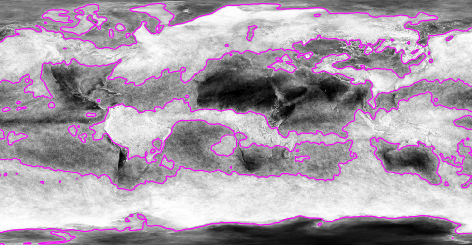 Since the contour polygons are GeoJSON, you can transform and display them using standard tools; see d3.geoPath, d3.geoProject and d3.geoStitch, for example.
Here the above contours of surface temperature are displayed in the Natural Earth projection:
Since the contour polygons are GeoJSON, you can transform and display them using standard tools; see d3.geoPath, d3.geoProject and d3.geoStitch, for example.
Here the above contours of surface temperature are displayed in the Natural Earth projection:
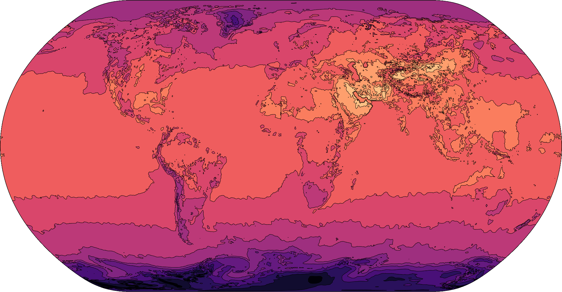 Contour plots can also visualize continuous functions by sampling.
Here is the Goldstein–Price function (a test function for global optimization) and a trippy animation of sin(x + y)sin(x - y):
Contour plots can also visualize continuous functions by sampling.
Here is the Goldstein–Price function (a test function for global optimization) and a trippy animation of sin(x + y)sin(x - y):
 Contours can also show the estimated density of point clouds, which is especially useful to avoid overplotting in large datasets.
This library implements fast two-dimensional kernel density estimation; see d3.contourDensity.
Here is a scatterplot showing the relationship between the idle duration and eruption duration for Old Faithful:
Contours can also show the estimated density of point clouds, which is especially useful to avoid overplotting in large datasets.
This library implements fast two-dimensional kernel density estimation; see d3.contourDensity.
Here is a scatterplot showing the relationship between the idle duration and eruption duration for Old Faithful:
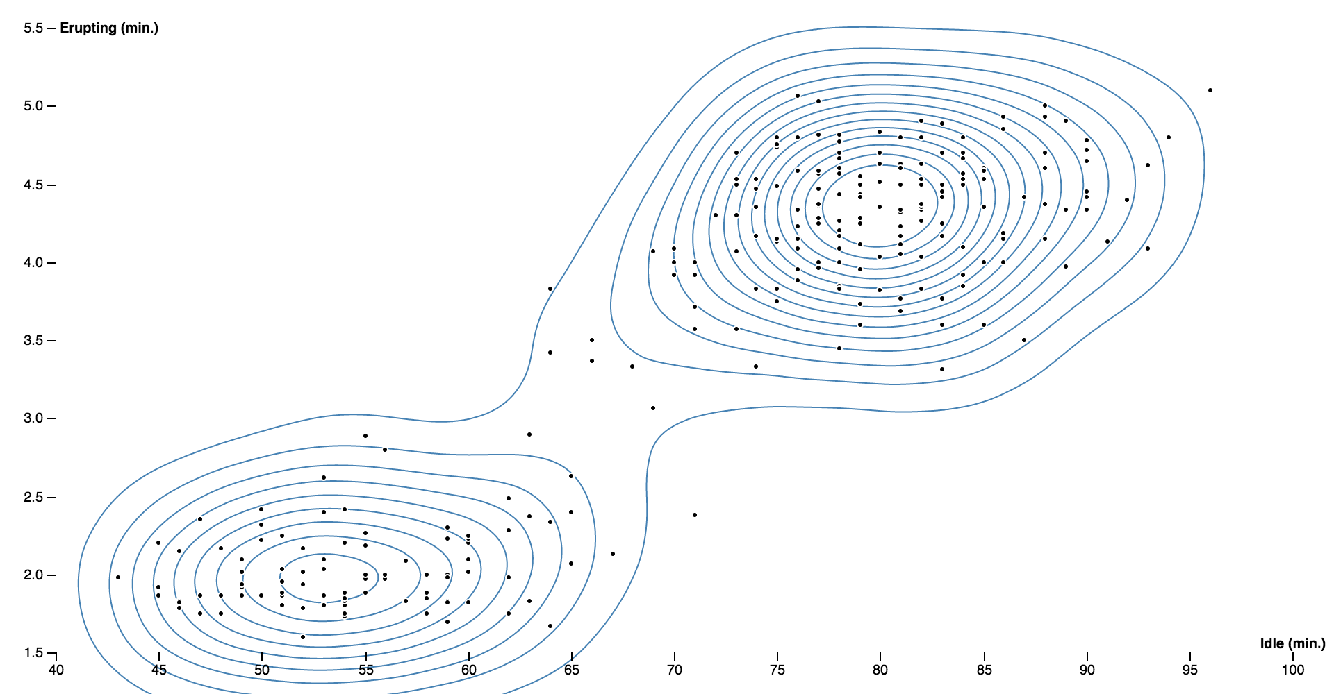 And here is a density contour plot showing the relationship between the weight and price of 53,940 diamonds:
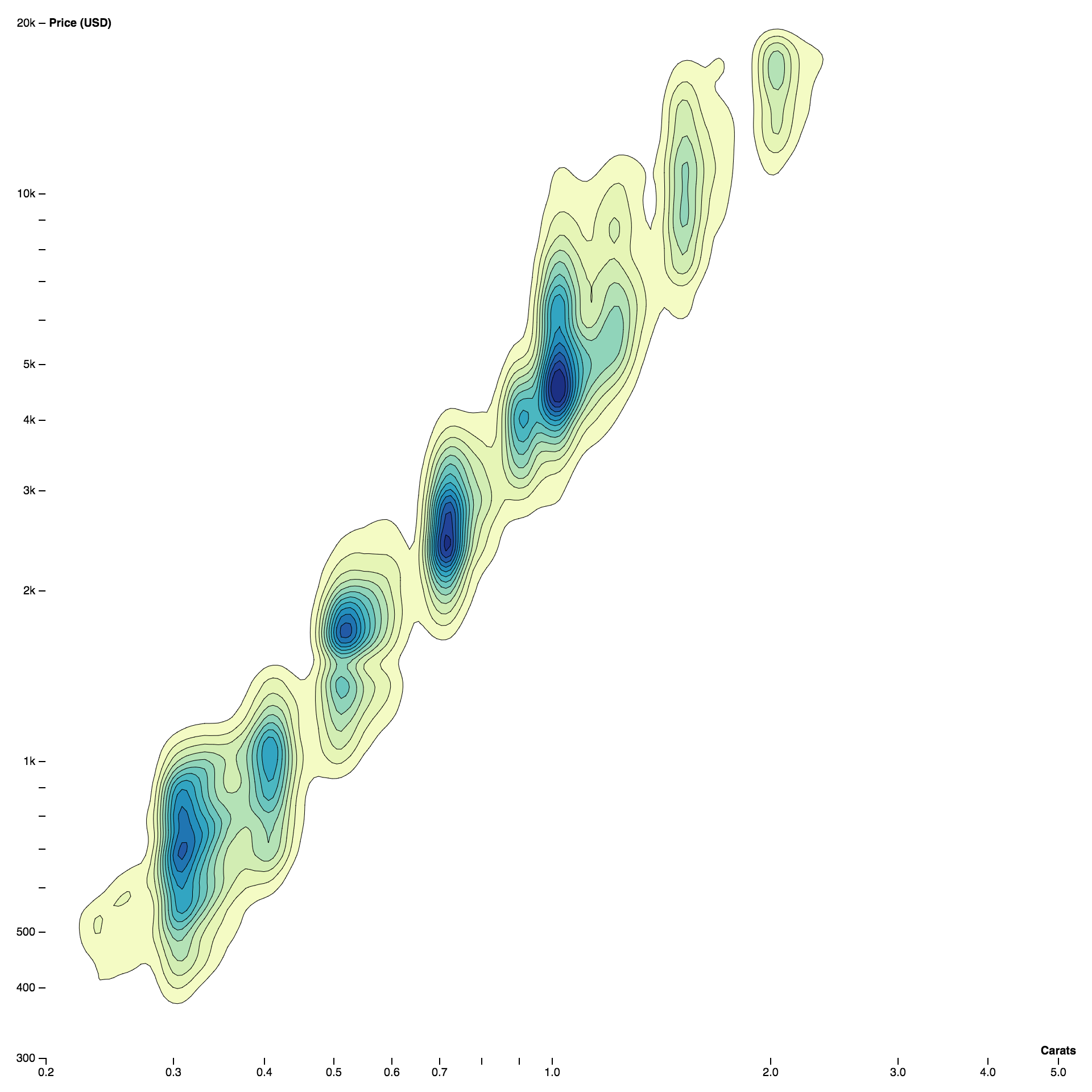
Installing
If you use NPM, npm install d3-contour.
Otherwise, download the latest release.
You can also load directly from d3js.org, either as a standalone library or as part of D3 4.0.
AMD, CommonJS, and vanilla environments are supported.
In vanilla, a d3 global is exported:
<script src="https://d3js.org/d3-array.v2.min.js"></script>
<script src="https://d3js.org/d3-contour.v2.min.js"></script>
<script>
// Populate a grid of n×m values where -2 = x = 2 and -2 = y = 1.
var n = 256, m = 256, values = new Array(n * m);
for (var j = 0.5, k = 0; j < m; ++j) {
for (var i = 0.5; i < n; ++i, ++k) {
values[k] = goldsteinPrice(i / n * 4 - 2, 1 - j / m * 3);
}
}
// Compute the contour polygons at log-spaced intervals; returns an array of MultiPolygon.
var contours = d3.contours()
.size([n, m])
.thresholds(d3.range(2, 21).map(p => Math.pow(2, p)))
(values);
// See https://en.wikipedia.org/wiki/Test_functions_for_optimization
function goldsteinPrice(x, y) {
return (1 + Math.pow(x + y + 1, 2) * (19 - 14 * x + 3 * x * x - 14 * y + 6 * x * x + 3 * y * y))
* (30 + Math.pow(2 * x - 3 * y, 2) * (18 - 32 * x + 12 * x * x + 48 * y - 36 * x * y + 27 * y * y));
}
</script>
API Reference
# d3.contours() <>
Constructs a new contour generator with the default settings.
# contours(values) <>
Computes the contours for the given array of values, returning an array of GeoJSON MultiPolygon geometry objects.
Each geometry object represents the area where the input values are greater than or equal to the corresponding threshold value; the threshold value for each geometry object is exposed as geometry.value.
The input values must be an array of length n×m where [n, m] is the contour generator’s size; furthermore, each values[i + jn] must represent the value at the position i, j.
For example, to construct a 256×256 grid for the Goldstein–Price function where -2 = x = 2 and -2 = y = 1:
var n = 256, m = 256, values = new Array(n * m);
for (var j = 0.5, k = 0; j < m; ++j) {
for (var i = 0.5; i < n; ++i, ++k) {
values[k] = goldsteinPrice(i / n * 4 - 2, 1 - j / m * 3);
}
}
function goldsteinPrice(x, y) {
return (1 + Math.pow(x + y + 1, 2) * (19 - 14 * x + 3 * x * x - 14 * y + 6 * x * x + 3 * y * y))
* (30 + Math.pow(2 * x - 3 * y, 2) * (18 - 32 * x + 12 * x * x + 48 * y - 36 * x * y + 27 * y * y));
}
The returned geometry objects are typically passed to d3.geoPath to display, using null or d3.geoIdentity as the associated projection.
# contours.contour(values, threshold) <>
Computes a single contour, returning a GeoJSON MultiPolygon geometry object representing the area where the input values are greater than or equal to the given threshold value; the threshold value for each geometry object is exposed as geometry.value.
The input values must be an array of length n×m where [n, m] is the contour generator’s size; furthermore, each values[i + jn] must represent the value at the position i, j.
See contours for an example.
# contours.size([size]) <>
If size is specified, sets the expected size of the input values grid to the contour generator and returns the contour generator.
The size is specified as an array [n, m] where n is the number of columns in the grid and m is the number of rows; n and m must be positive integers.
If size is not specified, returns the current size which defaults to [1, 1].
# contours.smooth([smooth]) <>
If smooth is specified, sets whether or not the generated contour polygons are smoothed using linear interpolation.
If smooth is not specified, returns the current smoothing flag, which defaults to true.
# contours.thresholds([thresholds]) <>
If thresholds is specified, sets the threshold generator to the specified function or array and returns this contour generator.
If thresholds is not specified, returns the current threshold generator, which by default implements Sturges’ formula.
Thresholds are defined as an array of values [x0, x1, …].
The first generated contour corresponds to the area where the input values are greater than or equal to x0; the second contour corresponds to the area where the input values are greater than or equal to x1, and so on.
Thus, there is exactly one generated MultiPolygon geometry object for each specified threshold value; the threshold value is exposed as geometry.value.
If a count is specified instead of an array of thresholds, then the input values’ extent will be uniformly divided into approximately count bins; see d3.ticks.
Density Estimation
# d3.contourDensity() <>
Constructs a new density estimator with the default settings.
# density(data) <>
Estimates the density contours for the given array of data, returning an array of GeoJSON MultiPolygon geometry objects.
Each geometry object represents the area where the estimated number of points per square pixel is greater than or equal to the corresponding threshold value; the threshold value for each geometry object is exposed as geometry.value.
The returned geometry objects are typically passed to d3.geoPath to display, using null or d3.geoIdentity as the associated projection.
See also d3.contours.
The x- and y-coordinate for each data point are computed using density.x and density.y.
In addition, density.weight indicates the relative contribution of each data point (default 1).
The generated contours are only accurate within the estimator’s defined size.
# density.x([x]) <>
If x is specified, sets the x-coordinate accessor.
If x is not specified, returns the current x-coordinate accessor, which defaults to:
function x(d) {
return d[0];
}
# density.y([y]) <>
If y is specified, sets the y-coordinate accessor.
If y is not specified, returns the current y-coordinate accessor, which defaults to:
function y(d) {
return d[1];
}
# density.weight([weight]) <>
If weight is specified, sets the accessor for point weights.
If weight is not specified, returns the current point weight accessor, which defaults to:
function weight() {
return 1;
}
# density.size([size]) <>
If size is specified, sets the size of the density estimator to the specified bounds and returns the estimator.
The size is specified as an array [width, height], where width is the maximum x-value and height is the maximum y-value.
If size is not specified, returns the current size which defaults to [960, 500].
The estimated density contours are only accurate within the defined size.
# density.cellSize([cellSize]) <>
If cellSize is specified, sets the size of individual cells in the underlying bin grid to the specified positive integer and returns the estimator.
If cellSize is not specified, returns the current cell size, which defaults to 4.
The cell size is rounded down to the nearest power of two.
Smaller cells produce more detailed contour polygons, but are more expensive to compute.
# density.thresholds([thresholds]) <>
If thresholds is specified, sets the threshold generator to the specified function or array and returns this contour generator.
If thresholds is not specified, returns the current threshold generator, which by default generates about twenty nicely-rounded density thresholds.
Thresholds are defined as an array of values [x0, x1, …].
The first generated density contour corresponds to the area where the estimated density is greater than or equal to x0; the second contour corresponds to the area where the estimated density is greater than or equal to x1, and so on.
Thus, there is exactly one generated MultiPolygon geometry object for each specified threshold value; the threshold value is exposed as geometry.value.
The first value x0 should typically be greater than zero.
If a count is specified instead of an array of thresholds, then approximately count uniformly-spaced nicely-rounded thresholds will be generated; see d3.ticks.
# density.bandwidth([bandwidth]) <>
If bandwidth is specified, sets the bandwidth (the standard deviation) of the Gaussian kernel and returns the estimate.
If bandwidth is not specified, returns the current bandwidth, which defaults to 20.4939….
The specified bandwidth is currently rounded to the nearest supported value by this implementation, and must be nonnegative.
d3-delaunay
 Georgy “The Voronator” Voronoy
This is a fast, no-dependency library for computing the Voronoi diagram of a set of two-dimensional points.
It is based on Delaunator, a fast library for computing the Delaunay triangulation using sweep algorithms.
The Voronoi diagram is constructed by connecting the circumcenters of adjacent triangles in the Delaunay triangulation.
For an interactive explanation of how this library works, see The Delaunay’s Dual.
Georgy “The Voronator” Voronoy
This is a fast, no-dependency library for computing the Voronoi diagram of a set of two-dimensional points.
It is based on Delaunator, a fast library for computing the Delaunay triangulation using sweep algorithms.
The Voronoi diagram is constructed by connecting the circumcenters of adjacent triangles in the Delaunay triangulation.
For an interactive explanation of how this library works, see The Delaunay’s Dual.
Installing
To install, npm install d3-delaunay or yarn add d3-delaunay.
You can also download the latest release or load directly from unpkg.
AMD, CommonJS and ES6+ environments are supported.
In vanilla, a d3 global is exported.
import {Delaunay} from "d3-delaunay";
const points = [[0, 0], [0, 1], [1, 0], [1, 1]];
const delaunay = Delaunay.from(points);
const voronoi = delaunay.voronoi([0, 0, 960, 500]);
API Reference
Delaunay
# new Delaunay(points) <>
Returns the Delaunay triangulation for the given flat array [x0, y0, x1, y1, …] of points.
const delaunay = new Delaunay(Float64Array.of(0, 0, 0, 1, 1, 0, 1, 1));
# Delaunay.from(points[, fx[, fy[, that]]]) <>
Returns the Delaunay triangulation for the given array or iterable of points.
If fx and fy are not specified, then points is assumed to be an array of two-element arrays of numbers: [[x0, y0], [x1, y1], …].
Otherwise, fx and fy are functions that are invoked for each element in the points array in order, and must return the respective x- and y-coordinate for each point.
If that is specified, the functions fx and fy are invoked with that as this.
(See Array.from for reference.)
const delaunay = Delaunay.from([[0, 0], [0, 1], [1, 0], [1, 1]]);
# delaunay.points
The coordinates of the points as an array [x0, y0, x1, y1, …].
Typically, this is a Float64Array, however you can use any array-like type in the constructor.
# delaunay.halfedges
The halfedge indexes as an Int32Array [j0, j1, …].
For each index 0 = i < halfedges.length, there is a halfedge from triangle vertex j = halfedges[i] to triangle vertex i.
Equivalently, this means that triangle i / 3 is adjacent to triangle j / 3.
If j is negative, then triangle i / 3 is an exterior triangle on the convex hull.
For example, to render the internal edges of the Delaunay triangulation:
const {points, halfedges, triangles} = delaunay;
for (let i = 0, n = halfedges.length; i < n; ++i) {
const j = halfedges[i];
if (j < i) continue;
const ti = triangles[i];
const tj = triangles[j];
context.moveTo(points[ti * 2], points[ti * 2 + 1]);
context.lineTo(points[tj * 2], points[tj * 2 + 1]);
}
See also delaunay.render.
# delaunay.hull
An Int32Array of point indexes that form the convex hull in counterclockwise order.
If the points are collinear, returns them ordered.
See also delaunay.renderHull.
# delaunay.triangles
The triangle vertex indexes as an Uint32Array [i0, j0, k0, i1, j1, k1, …].
Each contiguous triplet of indexes i, j, k forms a counterclockwise triangle.
The coordinates of the triangle’s points can be found by going through delaunay.points.
For example, to render triangle i:
const {points, triangles} = delaunay;
const t0 = triangles[i * 3 + 0];
const t1 = triangles[i * 3 + 1];
const t2 = triangles[i * 3 + 2];
context.moveTo(points[t0 * 2], points[t0 * 2 + 1]);
context.lineTo(points[t1 * 2], points[t1 * 2 + 1]);
context.lineTo(points[t2 * 2], points[t2 * 2 + 1]);
context.closePath();
See also delaunay.renderTriangle.
# delaunay.inedges
The incoming halfedge indexes as a Int32Array [e0, e1, e2, …].
For each point i, inedges[i] is the halfedge index e of an incoming halfedge.
For coincident points, the halfedge index is -1; for points on the convex hull, the incoming halfedge is on the convex hull; for other points, the choice of incoming halfedge is arbitrary.
The inedges table can be used to traverse the Delaunay triangulation; see also delaunay.neighbors.
# delaunay.find(x, y[, i]) <>
Returns the index of the input point that is closest to the specified point x, y.
The search is started at the specified point i.
If i is not specified, it defaults to zero.
# delaunay.neighbors(i) <>
Returns an iterable over the indexes of the neighboring points to the specified point i.
The iterable is empty if i is a coincident point.
# delaunay.render([context]) <>
 Renders the edges of the Delaunay triangulation to the specified context.
The specified context must implement the context.moveTo and context.lineTo methods from the CanvasPathMethods API.
If a context is not specified, an SVG path string is returned instead.
# delaunay.renderHull([context]) <>
Renders the edges of the Delaunay triangulation to the specified context.
The specified context must implement the context.moveTo and context.lineTo methods from the CanvasPathMethods API.
If a context is not specified, an SVG path string is returned instead.
# delaunay.renderHull([context]) <>
 Renders the convex hull of the Delaunay triangulation to the specified context.
The specified context must implement the context.moveTo and context.lineTo methods from the CanvasPathMethods API.
If a context is not specified, an SVG path string is returned instead.
# delaunay.renderTriangle(i[, context]) <>
Renders the convex hull of the Delaunay triangulation to the specified context.
The specified context must implement the context.moveTo and context.lineTo methods from the CanvasPathMethods API.
If a context is not specified, an SVG path string is returned instead.
# delaunay.renderTriangle(i[, context]) <>
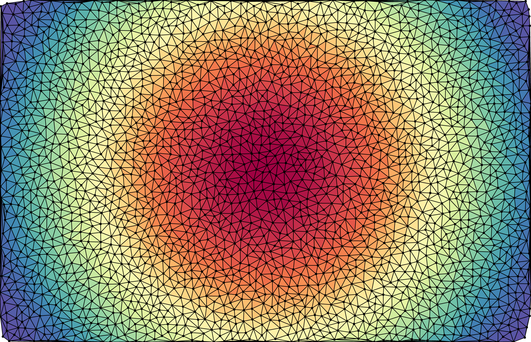 Renders triangle i of the Delaunay triangulation to the specified context.
The specified context must implement the context.moveTo, context.lineTo and context.closePath methods from the CanvasPathMethods API.
If a context is not specified, an SVG path string is returned instead.
# delaunay.renderPoints([context][, radius]) <>
Renders the input points of the Delaunay triangulation to the specified context as circles with the specified radius.
If radius is not specified, it defaults to 2.
The specified context must implement the context.moveTo and context.arc methods from the CanvasPathMethods API.
If a context is not specified, an SVG path string is returned instead.
# delaunay.hullPolygon() <>
Returns the closed polygon [[x0, y0], [x1, y1], …, [x0, y0]] representing the convex hull.
# delaunay.trianglePolygons() <>
Returns an iterable over the polygons for each triangle, in order.
# delaunay.trianglePolygon(i) <>
Returns the closed polygon [[x0, y0], [x1, y1], [x2, y2], [x0, y0]] representing the triangle i.
# delaunay.update() <>
Updates the triangulation after the points have been modified in-place.
# delaunay.voronoi([bounds]) <>
Returns the Voronoi diagram for the associated points.
When rendering, the diagram will be clipped to the specified bounds = [xmin, ymin, xmax, ymax].
If bounds is not specified, it defaults to [0, 0, 960, 500].
See To Infinity and Back Again for an interactive explanation of Voronoi cell clipping.
The Voronoi diagram is returned even in degenerate cases where no triangulation exists — namely 0, 1 or 2 points, and collinear points.
Renders triangle i of the Delaunay triangulation to the specified context.
The specified context must implement the context.moveTo, context.lineTo and context.closePath methods from the CanvasPathMethods API.
If a context is not specified, an SVG path string is returned instead.
# delaunay.renderPoints([context][, radius]) <>
Renders the input points of the Delaunay triangulation to the specified context as circles with the specified radius.
If radius is not specified, it defaults to 2.
The specified context must implement the context.moveTo and context.arc methods from the CanvasPathMethods API.
If a context is not specified, an SVG path string is returned instead.
# delaunay.hullPolygon() <>
Returns the closed polygon [[x0, y0], [x1, y1], …, [x0, y0]] representing the convex hull.
# delaunay.trianglePolygons() <>
Returns an iterable over the polygons for each triangle, in order.
# delaunay.trianglePolygon(i) <>
Returns the closed polygon [[x0, y0], [x1, y1], [x2, y2], [x0, y0]] representing the triangle i.
# delaunay.update() <>
Updates the triangulation after the points have been modified in-place.
# delaunay.voronoi([bounds]) <>
Returns the Voronoi diagram for the associated points.
When rendering, the diagram will be clipped to the specified bounds = [xmin, ymin, xmax, ymax].
If bounds is not specified, it defaults to [0, 0, 960, 500].
See To Infinity and Back Again for an interactive explanation of Voronoi cell clipping.
The Voronoi diagram is returned even in degenerate cases where no triangulation exists — namely 0, 1 or 2 points, and collinear points.
Voronoi
# voronoi.delaunay
The Voronoi diagram’s associated Delaunay triangulation.
# voronoi.circumcenters
The circumcenters of the Delaunay triangles as a Float64Array [cx0, cy0, cx1, cy1, …].
Each contiguous pair of coordinates cx, cy is the circumcenter for the corresponding triangle.
These circumcenters form the coordinates of the Voronoi cell polygons.
# voronoi.vectors
A Float64Array [vx0, vy0, wx0, wy0, …] where each non-zero quadruple describes an open (infinite) cell on the outer hull, giving the directions of two open half-lines.
# voronoi.xmin
# voronoi.ymin
# voronoi.xmax
# voronoi.ymax
The bounds of the viewport [xmin, ymin, xmax, ymax] for rendering the Voronoi diagram.
These values only affect the rendering methods (voronoi.render, voronoi.renderBounds, cell.render).
# voronoi.contains(i, x, y) <>
Returns true if the cell with the specified index i contains the specified point x, y.
(This method is not affected by the associated Voronoi diagram’s viewport bounds.)
# voronoi.neighbors(i) <>
Returns an iterable over the indexes of the cells that share a common edge with the specified cell i.
Voronoi neighbors are always neighbors on the Delaunay graph, but the converse is false when the common edge has been clipped out by the Voronoi diagram’s viewport.
# voronoi.render([context]) <>
 Renders the mesh of Voronoi cells to the specified context.
The specified context must implement the context.moveTo and context.lineTo methods from the CanvasPathMethods API.
If a context is not specified, an SVG path string is returned instead.
# voronoi.renderBounds([context]) <>
Renders the mesh of Voronoi cells to the specified context.
The specified context must implement the context.moveTo and context.lineTo methods from the CanvasPathMethods API.
If a context is not specified, an SVG path string is returned instead.
# voronoi.renderBounds([context]) <>
 Renders the viewport extent to the specified context.
The specified context must implement the context.rect method from the CanvasPathMethods API.
Equivalent to context.rect(voronoi.xmin, voronoi.ymin, voronoi.xmax - voronoi.xmin, voronoi.ymax - voronoi.ymin).
If a context is not specified, an SVG path string is returned instead.
# voronoi.renderCell(i[, context]) <>
Renders the viewport extent to the specified context.
The specified context must implement the context.rect method from the CanvasPathMethods API.
Equivalent to context.rect(voronoi.xmin, voronoi.ymin, voronoi.xmax - voronoi.xmin, voronoi.ymax - voronoi.ymin).
If a context is not specified, an SVG path string is returned instead.
# voronoi.renderCell(i[, context]) <>
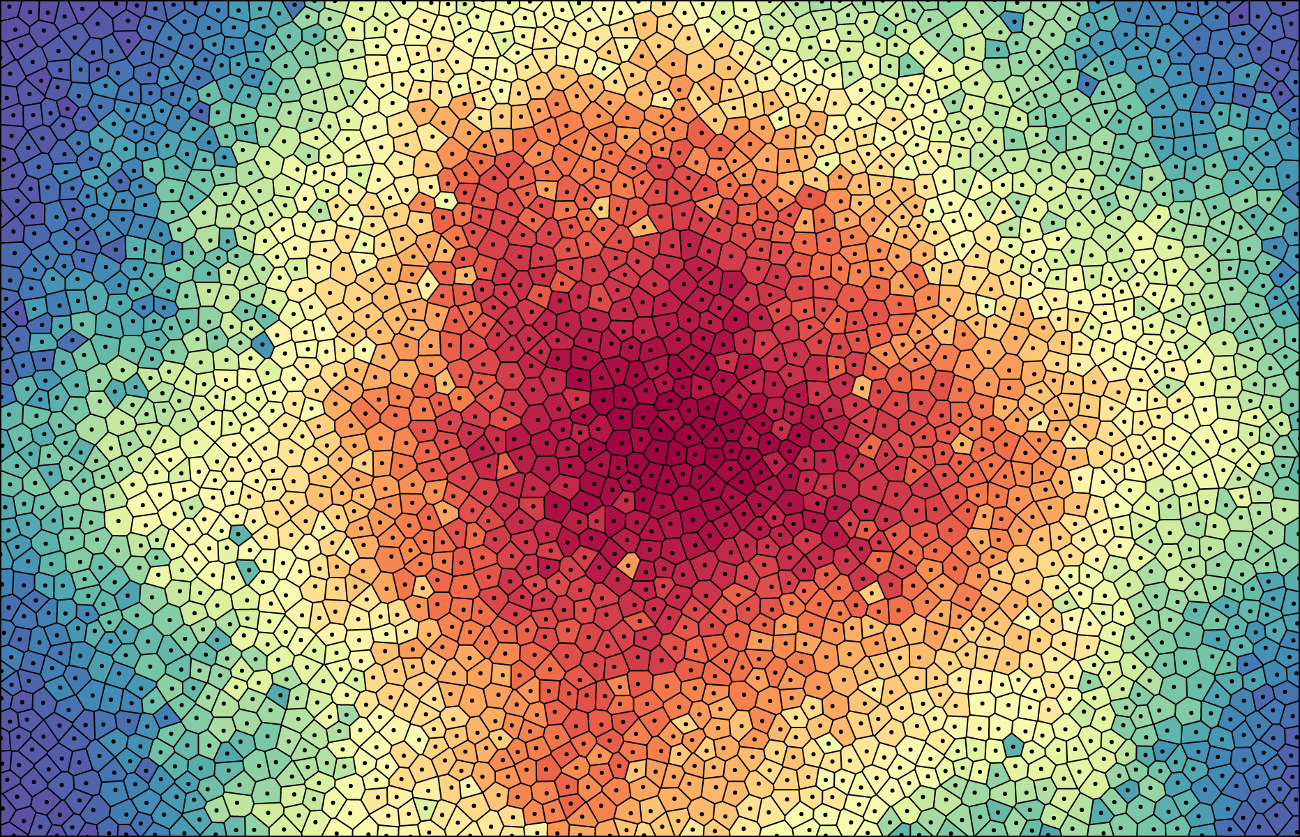 Renders the cell with the specified index i to the specified context.
The specified context must implement the context.moveTo , context.lineTo and context.closePath methods from the CanvasPathMethods API.
If a context is not specified, an SVG path string is returned instead.
# voronoi.cellPolygons() <>
Returns an iterable over the non-empty polygons for each cell, with the cell index as property.
# voronoi.cellPolygon(i) <>
Returns the convex, closed polygon [[x0, y0], [x1, y1], …, [x0, y0]] representing the cell for the specified point i.
# voronoi.update() <>
Updates the Voronoi diagram and underlying triangulation after the points have been modified in-place — useful for Lloyd’s relaxation.
Renders the cell with the specified index i to the specified context.
The specified context must implement the context.moveTo , context.lineTo and context.closePath methods from the CanvasPathMethods API.
If a context is not specified, an SVG path string is returned instead.
# voronoi.cellPolygons() <>
Returns an iterable over the non-empty polygons for each cell, with the cell index as property.
# voronoi.cellPolygon(i) <>
Returns the convex, closed polygon [[x0, y0], [x1, y1], …, [x0, y0]] representing the cell for the specified point i.
# voronoi.update() <>
Updates the Voronoi diagram and underlying triangulation after the points have been modified in-place — useful for Lloyd’s relaxation.
d3-dispatch
Dispatching is a convenient mechanism for separating concerns with loosely-coupled code: register named callbacks and then call them with arbitrary arguments.
A variety of D3 components, such as d3-request, use this mechanism to emit events to listeners.
Think of this like Node’s EventEmitter, except every listener has a well-defined name so it’s easy to remove or replace them.
For example, to create a dispatch for start and end events:
var dispatch = d3.dispatch("start", "end");
You can then register callbacks for these events using dispatch.on:
dispatch.on("start", callback1);
dispatch.on("start.foo", callback2);
dispatch.on("end", callback3);
Then, you can invoke all the start callbacks using dispatch.call or dispatch.apply:
dispatch.call("start");
Like function.call, you may also specify the this context and any arguments:
dispatch.call("start", {about: "I am a context object"}, "I am an argument");
Want a more involved example? See how to use d3-dispatch for coordinated views.
Installing
If you use NPM, npm install d3-dispatch.
Otherwise, download the latest release.
You can also load directly from d3js.org, either as a standalone library or as part of D3.
AMD, CommonJS, and vanilla environments are supported.
In vanilla, a d3 global is exported:
<script src="https://d3js.org/d3-dispatch.v1.min.js"></script>
<script>
var dispatch = d3.dispatch("start", "end");
</script>
Try d3-dispatch in your browser.
API Reference
# d3.dispatch(types…) · Source
Creates a new dispatch for the specified event types.
Each type is a string, such as "start" or "end".
# dispatch.on(typenames[, callback]) · Source
Adds, removes or gets the callback for the specified typenames.
If a callback function is specified, it is registered for the specified (fully-qualified) typenames.
If a callback was already registered for the given typenames, the existing callback is removed before the new callback is added.
The specified typenames is a string, such as start or end.foo.
The type may be optionally followed by a period (.) and a name; the optional name allows multiple callbacks to be registered to receive events of the same type, such as start.foo and start.bar.
To specify multiple typenames, separate typenames with spaces, such as start end or start.foo start.bar.
To remove all callbacks for a given name foo, say dispatch.on(".foo", null).
If callback is not specified, returns the current callback for the specified typenames, if any.
If multiple typenames are specified, the first matching callback is returned.
# dispatch.copy() · Source
Returns a copy of this dispatch object.
Changes to this dispatch do not affect the returned copy and vice versa.
# dispatch.call(type[, that[, arguments…]]) · Source
Like function.call, invokes each registered callback for the specified type, passing the callback the specified arguments, with that as the this context.
See dispatch.apply for more information.
# dispatch.apply(type[, that[, arguments]]) · Source
Like function.apply, invokes each registered callback for the specified type, passing the callback the specified arguments, with that as the this context.
For example, if you wanted to dispatch your custom callbacks after handling a native click event, while preserving the current this context and arguments, you could say:
selection.on("click", function() {
dispatch.apply("custom", this, arguments);
});
You can pass whatever arguments you want to callbacks; most commonly, you might create an object that represents an event, or pass the current datum (d) and index (i).
See function.call and function.apply for further information.
d3-drag
Drag-and-drop is a popular and easy-to-learn pointing gesture: move the pointer to an object, press and hold to grab it, “drag” the object to a new location, and release to “drop”.
D3’s drag behavior provides a convenient but flexible abstraction for enabling drag-and-drop interaction on selections.
For example, you can use d3-drag to facilitate interaction with a force-directed graph, or a simulation of colliding circles:
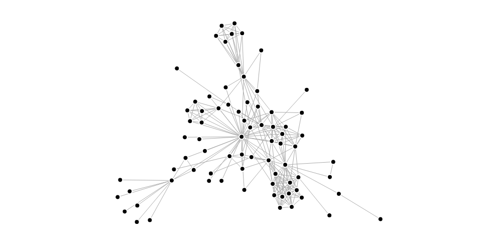
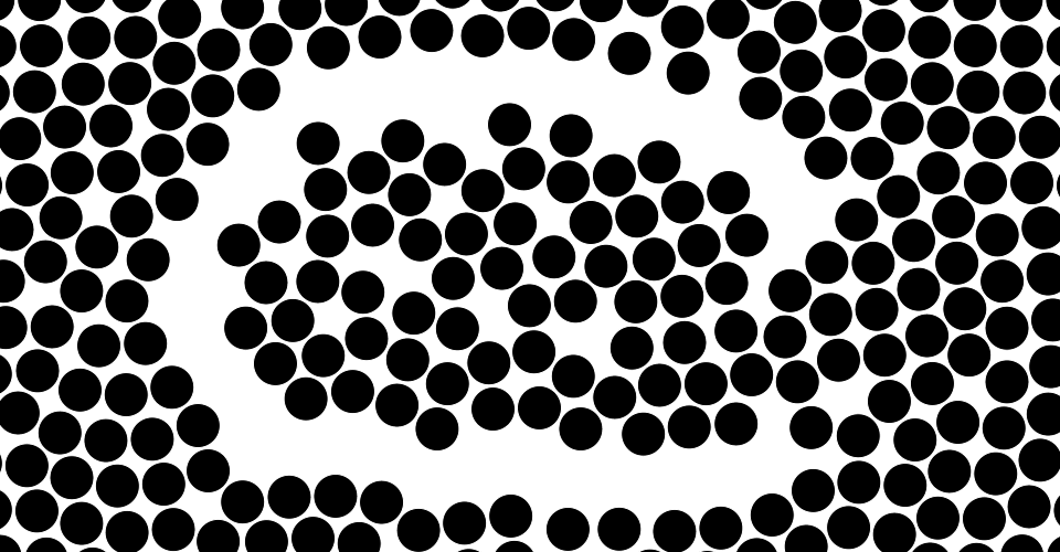 You can also use d3-drag to implement custom user interface elements, such as a slider.
But the drag behavior isn’t just for moving elements around; there are a variety of ways to respond to a drag gesture.
For example, you can use it to lasso elements in a scatterplot, or to paint lines on a canvas:
You can also use d3-drag to implement custom user interface elements, such as a slider.
But the drag behavior isn’t just for moving elements around; there are a variety of ways to respond to a drag gesture.
For example, you can use it to lasso elements in a scatterplot, or to paint lines on a canvas:
 The drag behavior can be combined with other behaviors, such as d3-zoom for zooming.
 The drag behavior is agnostic about the DOM, so you can use it with SVG, HTML or even Canvas! And you can extend it with advanced selection techniques, such as a Voronoi overlay or a closest-target search:
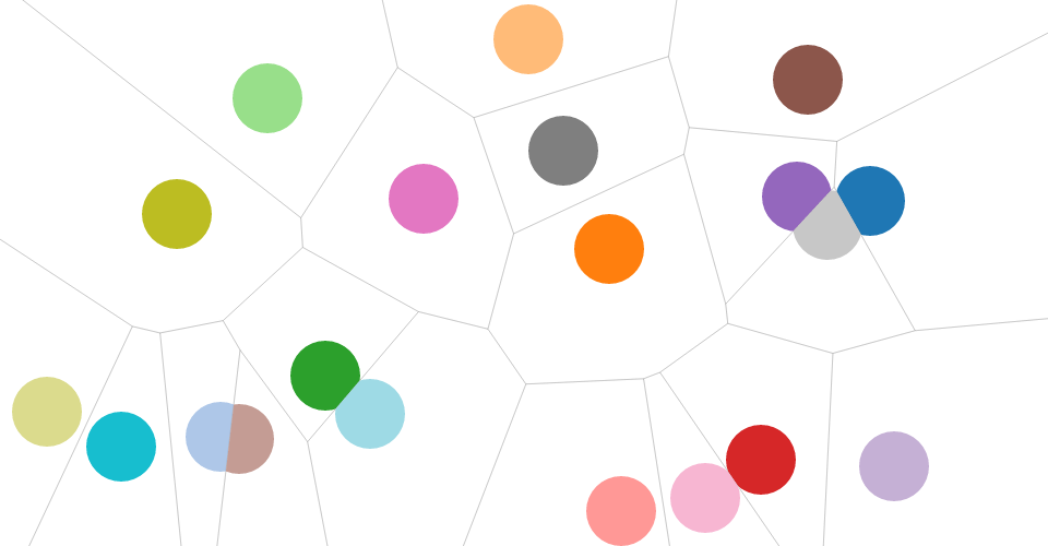
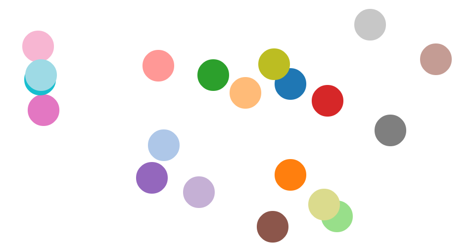 Best of all, the drag behavior automatically unifies mouse and touch input, and avoids browser idiosyncrasies.
When Pointer Events are more widely available, the drag behavior will support those, too.
Best of all, the drag behavior automatically unifies mouse and touch input, and avoids browser idiosyncrasies.
When Pointer Events are more widely available, the drag behavior will support those, too.
Installing
If you use NPM, npm install d3-drag.
Otherwise, download the latest release.
You can also load directly from d3js.org, either as a standalone library or as part of D3.
AMD, CommonJS, and vanilla environments are supported.
In vanilla, a d3 global is exported:
<script src="https://d3js.org/d3-dispatch.v2.min.js"></script>
<script src="https://d3js.org/d3-selection.v2.min.js"></script>
<script src="https://d3js.org/d3-drag.v2.min.js"></script>
<script>
var drag = d3.drag();
</script>
Try d3-drag in your browser.
API Reference
This table describes how the drag behavior interprets native events:
| Event |
Listening Element |
Drag Event |
Default Prevented? |
| mousedown5 |
selection |
start |
no¹ |
| mousemove² |
window¹ |
drag |
yes |
| mouseup² |
window¹ |
end |
yes |
| dragstart² |
window |
- |
yes |
| selectstart² |
window |
- |
yes |
| click³ |
window |
- |
yes |
| touchstart |
selection |
start |
no4 |
| touchmove |
selection |
drag |
yes |
| touchend |
selection |
end |
no4 |
| touchcancel |
selection |
end |
no4 |
The propagation of all consumed events is immediately stopped.
If you want to prevent some events from initiating a drag gesture, use drag.filter.
¹ Necessary to capture events outside an iframe; see #9.
² Only applies during an active, mouse-based gesture; see #9.
³ Only applies immediately after some mouse-based gestures; see drag.clickDistance.
4 Necessary to allow click emulation on touch input; see #9.
5 Ignored if within 500ms of a touch gesture ending; assumes click emulation.
# d3.drag() · Source, Examples
Creates a new drag behavior.
The returned behavior, drag, is both an object and a function, and is typically applied to selected elements via selection.call.
# drag(selection) · Source, Examples
Applies this drag behavior to the specified selection.
This function is typically not invoked directly, and is instead invoked via selection.call.
For example, to instantiate a drag behavior and apply it to a selection:
d3.selectAll(".node").call(d3.drag().on("start", started));
Internally, the drag behavior uses selection.on to bind the necessary event listeners for dragging.
The listeners use the name .drag, so you can subsequently unbind the drag behavior as follows:
selection.on(".drag", null);
Applying the drag behavior also sets the -webkit-tap-highlight-color style to transparent, disabling the tap highlight on iOS.
If you want a different tap highlight color, remove or re-apply this style after applying the drag behavior.
# drag.container([container]) · Source, Examples
If container is specified, sets the container accessor to the specified object or function and returns the drag behavior.
If container is not specified, returns the current container accessor, which defaults to:
function container() {
return this.parentNode;
}
The container of a drag gesture determines the coordinate system of subsequent drag events, affecting event.x and event.y.
The element returned by the container accessor is subsequently passed to d3.pointer to determine the local coordinates of the pointer.
The default container accessor returns the parent node of the element in the originating selection (see drag) that received the initiating input event.
This is often appropriate when dragging SVG or HTML elements, since those elements are typically positioned relative to a parent.
For dragging graphical elements with a Canvas, however, you may want to redefine the container as the initiating element itself:
function container() {
return this;
}
Alternatively, the container may be specified as the element directly, such as drag.container(canvas).
# drag.filter([filter]) · Source, Examples
If filter is specified, sets the event filter to the specified function and returns the drag behavior.
If filter is not specified, returns the current filter, which defaults to:
function filter(event) {
return !event.ctrlKey && !event.button;
}
If the filter returns falsey, the initiating event is ignored and no drag gestures are started.
Thus, the filter determines which input events are ignored; the default filter ignores mousedown events on secondary buttons, since those buttons are typically intended for other purposes, such as the context menu.
# drag.touchable([touchable]) · Source, Examples
If touchable is specified, sets the touch support detector to the specified function and returns the drag behavior.
If touchable is not specified, returns the current touch support detector, which defaults to:
function touchable() {
return navigator.maxTouchPoints || ("ontouchstart" in this);
}
Touch event listeners are only registered if the detector returns truthy for the corresponding element when the drag behavior is applied.
The default detector works well for most browsers that are capable of touch input, but not all; Chrome’s mobile device emulator, for example, fails detection.
# drag.subject([subject]) · Source, Examples
If subject is specified, sets the subject accessor to the specified object or function and returns the drag behavior.
If subject is not specified, returns the current subject accessor, which defaults to:
function subject(event, d) {
return d == null ? {x: event.x, y: event.y} : d;
}
The subject of a drag gesture represents the thing being dragged.
It is computed when an initiating input event is received, such as a mousedown or touchstart, immediately before the drag gesture starts.
The subject is then exposed as event.subject on subsequent drag events for this gesture.
The default subject is the datum of the element in the originating selection (see drag) that received the initiating input event; if this datum is undefined, an object representing the coordinates of the pointer is created.
When dragging circle elements in SVG, the default subject is thus the datum of the circle being dragged.
With Canvas, the default subject is the canvas element’s datum (regardless of where on the canvas you click).
In this case, a custom subject accessor would be more appropriate, such as one that picks the closest circle to the mouse within a given search radius:
function subject(event) {
var n = circles.length,
i,
dx,
dy,
d2,
s2 = radius * radius,
circle,
subject;
for (i = 0; i < n; ++i) {
circle = circles[i];
dx = event.x - circle.x;
dy = event.y - circle.y;
d2 = dx * dx + dy * dy;
if (d2 < s2) subject = circle, s2 = d2;
}
return subject;
}
(If necessary, the above can be accelerated using quadtree.find, simulation.find or delaunay.find.)
The returned subject should be an object that exposes x and y properties, so that the relative position of the subject and the pointer can be preserved during the drag gesture.
If the subject is null or undefined, no drag gesture is started for this pointer; however, other starting touches may yet start drag gestures.
See also drag.filter.
The subject of a drag gesture may not be changed after the gesture starts.
The subject accessor is invoked with the same context and arguments as selection.on listeners: the current event (event) and datum d, with the this context as the current DOM element.
During the evaluation of the subject accessor, event is a beforestart drag event.
Use event.sourceEvent to access the initiating input event and event.identifier to access the touch identifier.
The event.x and event.y are relative to the container, and are computed using d3.pointer.
# drag.clickDistance([distance]) · Source
If distance is specified, sets the maximum distance that the mouse can move between mousedown and mouseup that will trigger a subsequent click event.
If at any point between mousedown and mouseup the mouse is greater than or equal to distance from its position on mousedown, the click event following mouseup will be suppressed.
If distance is not specified, returns the current distance threshold, which defaults to zero.
The distance threshold is measured in client coordinates (event.clientX and event.clientY).
# drag.on(typenames, [listener]) · Source
If listener is specified, sets the event listener for the specified typenames and returns the drag behavior.
If an event listener was already registered for the same type and name, the existing listener is removed before the new listener is added.
If listener is null, removes the current event listeners for the specified typenames, if any.
If listener is not specified, returns the first currently-assigned listener matching the specified typenames, if any.
When a specified event is dispatched, each listener will be invoked with the same context and arguments as selection.on listeners: the current event (event) and datum d, with the this context as the current DOM element.
The typenames is a string containing one or more typename separated by whitespace.
Each typename is a type, optionally followed by a period (.) and a name, such as drag.foo and drag.bar; the name allows multiple listeners to be registered for the same type.
The type must be one of the following:
start - after a new pointer becomes active (on mousedown or touchstart).
drag - after an active pointer moves (on mousemove or touchmove).
end - after an active pointer becomes inactive (on mouseup, touchend or touchcancel).
See dispatch.on for more.
Changes to registered listeners via drag.on during a drag gesture do not affect the current drag gesture.
Instead, you must use event.on, which also allows you to register temporary event listeners for the current drag gesture.
Separate events are dispatched for each active pointer during a drag gesture.
For example, if simultaneously dragging multiple subjects with multiple fingers, a start event is dispatched for each finger, even if both fingers start touching simultaneously.
See Drag Events for more.
# d3.dragDisable(window) · Source
Prevents native drag-and-drop and text selection on the specified window.
As an alternative to preventing the default action of mousedown events (see #9), this method prevents undesirable default actions following mousedown.
In supported browsers, this means capturing dragstart and selectstart events, preventing the associated default actions, and immediately stopping their propagation.
In browsers that do not support selection events, the user-select CSS property is set to none on the document element.
This method is intended to be called on mousedown, followed by d3.dragEnable on mouseup.
# d3.dragEnable(window[, noclick]) · Source
Allows native drag-and-drop and text selection on the specified window; undoes the effect of d3.dragDisable.
This method is intended to be called on mouseup, preceded by d3.dragDisable on mousedown.
If noclick is true, this method also temporarily suppresses click events.
The suppression of click events expires after a zero-millisecond timeout, such that it only suppress the click event that would immediately follow the current mouseup event, if any.
Drag Events
When a drag event listener is invoked, it receives the current drag event as its first argument.
The event object exposes several fields:
target - the associated drag behavior.
type - the string “start”, “drag” or “end”; see drag.on.
subject - the drag subject, defined by drag.subject.
x - the new x-coordinate of the subject; see drag.container.
y - the new y-coordinate of the subject; see drag.container.
dx - the change in x-coordinate since the previous drag event.
dy - the change in y-coordinate since the previous drag event.
identifier - the string “mouse”, or a numeric touch identifier.
active - the number of currently active drag gestures (on start and end, not including this one).
sourceEvent - the underlying input event, such as mousemove or touchmove.
The event.active field is useful for detecting the first start event and the last end event in a sequence of concurrent drag gestures: it is zero when the first drag gesture starts, and zero when the last drag gesture ends.
The event object also exposes the event.on method.
# event.on(typenames, [listener]) · Source
Equivalent to drag.on, but only applies to the current drag gesture.
Before the drag gesture starts, a copy of the current drag event listeners is made.
This copy is bound to the current drag gesture and modified by event.on.
This is useful for temporary listeners that only receive events for the current drag gesture.
For example, this start event listener registers temporary drag and end event listeners as closures:
function started(event) {
var circle = d3.select(this).classed("dragging", true);
event.on("drag", dragged).on("end", ended);
function dragged(event, d) {
circle.raise().attr("cx", d.x = event.x).attr("cy", d.y = event.y);
}
function ended() {
circle.classed("dragging", false);
}
}
d3-dsv
This module provides a parser and formatter for delimiter-separated values, most commonly comma- (CSV) or tab-separated values (TSV).
These tabular formats are popular with spreadsheet programs such as Microsoft Excel, and are often more space-efficient than JSON.
This implementation is based on RFC 4180.
Comma (CSV) and tab (TSV) delimiters are built-in.
For example, to parse:
d3.csvParse("foo,bar\n1,2"); // [{foo: "1", bar: "2"}, columns: ["foo", "bar"]]
d3.tsvParse("foo\tbar\n1\t2"); // [{foo: "1", bar: "2"}, columns: ["foo", "bar"]]
Or to format:
d3.csvFormat([{foo: "1", bar: "2"}]); // "foo,bar\n1,2"
d3.tsvFormat([{foo: "1", bar: "2"}]); // "foo\tbar\n1\t2"
To use a different delimiter, such as “|” for pipe-separated values, use d3.dsvFormat:
var psv = d3.dsvFormat("|");
console.log(psv.parse("foo|bar\n1|2")); // [{foo: "1", bar: "2"}, columns: ["foo", "bar"]]
For easy loading of DSV files in a browser, see d3-fetch’s d3.csv and d3.tsv methods.
Installing
If you use NPM, npm install d3-dsv.
Otherwise, download the latest release.
You can also load directly from d3js.org, either as a standalone library or as part of D3.
AMD, CommonJS, and vanilla environments are supported.
In vanilla, a d3 global is exported:
<script src="https://d3js.org/d3-dsv.v1.min.js"></script>
<script>
var data = d3.csvParse(string);
</script>
Try d3-dsv in your browser.
API Reference
# d3.csvParse(string[, row]) <>
Equivalent to dsvFormat(",").parse.
Note: requires unsafe-eval content security policy.
# d3.csvParseRows(string[, row]) <>
Equivalent to dsvFormat(",").parseRows.
# d3.csvFormat(rows[, columns]) <>
Equivalent to dsvFormat(",").format.
# d3.csvFormatBody(rows[, columns]) <>
Equivalent to dsvFormat(",").formatBody.
# d3.csvFormatRows(rows) <>
Equivalent to dsvFormat(",").formatRows.
# d3.csvFormatRow(row) <>
Equivalent to dsvFormat(",").formatRow.
# d3.csvFormatValue(value) <>
Equivalent to dsvFormat(",").formatValue.
# d3.tsvParse(string[, row]) <>
Equivalent to dsvFormat("\t").parse.
Note: requires unsafe-eval content security policy.
# d3.tsvParseRows(string[, row]) <>
Equivalent to dsvFormat("\t").parseRows.
# d3.tsvFormat(rows[, columns]) <>
Equivalent to dsvFormat("\t").format.
# d3.tsvFormatBody(rows[, columns]) <>
Equivalent to dsvFormat("\t").formatBody.
# d3.tsvFormatRows(rows) <>
Equivalent to dsvFormat("\t").formatRows.
# d3.tsvFormatRow(row) <>
Equivalent to dsvFormat("\t").formatRow.
# d3.tsvFormatValue(value) <>
Equivalent to dsvFormat("\t").formatValue.
# d3.dsvFormat(delimiter) <>
Constructs a new DSV parser and formatter for the specified delimiter.
The delimiter must be a single character (i.e., a single 16-bit code unit); so, ASCII delimiters are fine, but emoji delimiters are not.
# dsv.parse(string[, row]) <>
Parses the specified string, which must be in the delimiter-separated values format with the appropriate delimiter, returning an array of objects representing the parsed rows.
Unlike dsv.parseRows, this method requires that the first line of the DSV content contains a delimiter-separated list of column names; these column names become the attributes on the returned objects.
For example, consider the following CSV file:
Year,Make,Model,Length
1997,Ford,E350,2.34
2000,Mercury,Cougar,2.38
The resulting JavaScript array is:
[
{"Year": "1997", "Make": "Ford", "Model": "E350", "Length": "2.34"},
{"Year": "2000", "Make": "Mercury", "Model": "Cougar", "Length": "2.38"}
]
The returned array also exposes a columns property containing the column names in input order (in contrast to Object.keys, whose iteration order is arbitrary).
For example:
data.columns; // ["Year", "Make", "Model", "Length"]
If the column names are not unique, only the last value is returned for each name; to access all values, use dsv.parseRows instead (see example).
If a row conversion function is not specified, field values are strings.
For safety, there is no automatic conversion to numbers, dates, or other types.
In some cases, JavaScript may coerce strings to numbers for you automatically (for example, using the + operator), but better is to specify a row conversion function.
See d3.autoType for a convenient row conversion function that infers and coerces common types like numbers and strings.
If a row conversion function is specified, the specified function is invoked for each row, being passed an object representing the current row (d), the index (i) starting at zero for the first non-header row, and the array of column names.
If the returned value is null or undefined, the row is skipped and will be omitted from the array returned by dsv.parse; otherwise, the returned value defines the corresponding row object.
For example:
var data = d3.csvParse(string, function(d) {
return {
year: new Date(+d.Year, 0, 1), // lowercase and convert "Year" to Date
make: d.Make, // lowercase
model: d.Model, // lowercase
length: +d.Length // lowercase and convert "Length" to number
};
});
Note: using + rather than parseInt or parseFloat is typically faster, though more restrictive.
For example, "30px" when coerced using + returns NaN, while parseInt and parseFloat return 30.
Note: requires unsafe-eval content security policy.
# dsv.parseRows(string[, row]) <>
Parses the specified string, which must be in the delimiter-separated values format with the appropriate delimiter, returning an array of arrays representing the parsed rows.
Unlike dsv.parse, this method treats the header line as a standard row, and should be used whenever DSV content does not contain a header.
Each row is represented as an array rather than an object.
Rows may have variable length.
For example, consider the following CSV file, which notably lacks a header line:
1997,Ford,E350,2.34
2000,Mercury,Cougar,2.38
The resulting JavaScript array is:
[
["1997", "Ford", "E350", "2.34"],
["2000", "Mercury", "Cougar", "2.38"]
]
If a row conversion function is not specified, field values are strings.
For safety, there is no automatic conversion to numbers, dates, or other types.
In some cases, JavaScript may coerce strings to numbers for you automatically (for example, using the + operator), but better is to specify a row conversion function.
See d3.autoType for a convenient row conversion function that infers and coerces common types like numbers and strings.
If a row conversion function is specified, the specified function is invoked for each row, being passed an array representing the current row (d), the index (i) starting at zero for the first row, and the array of column names.
If the returned value is null or undefined, the row is skipped and will be omitted from the array returned by dsv.parse; otherwise, the returned value defines the corresponding row object.
For example:
var data = d3.csvParseRows(string, function(d, i) {
return {
year: new Date(+d[0], 0, 1), // convert first colum column to Date
make: d[1],
model: d[2],
length: +d[3] // convert fourth column to number
};
});
In effect, row is similar to applying a map and filter operator to the returned rows.
# dsv.format(rows[, columns]) <>
Formats the specified array of object rows as delimiter-separated values, returning a string.
This operation is the inverse of dsv.parse.
Each row will be separated by a newline (\n), and each column within each row will be separated by the delimiter (such as a comma, ,).
Values that contain either the delimiter, a double-quote (") or a newline will be escaped using double-quotes.
If columns is not specified, the list of column names that forms the header row is determined by the union of all properties on all objects in rows; the order of columns is nondeterministic.
If columns is specified, it is an array of strings representing the column names.
For example:
var string = d3.csvFormat(data, ["year", "make", "model", "length"]);
All fields on each row object will be coerced to strings.
If the field value is null or undefined, the empty string is used.
If the field value is a Date, the ECMAScript date-time string format (a subset of ISO 8601) is used: for example, dates at UTC midnight are formatted as YYYY-MM-DD.
For more control over which and how fields are formatted, first map rows to an array of array of string, and then use dsv.formatRows.
# dsv.formatBody(rows[, columns]) <>
Equivalent to dsv.format, but omits the header row.
This is useful, for example, when appending rows to an existing file.
# dsv.formatRows(rows) <>
Formats the specified array of array of string rows as delimiter-separated values, returning a string.
This operation is the reverse of dsv.parseRows.
Each row will be separated by a newline (\n), and each column within each row will be separated by the delimiter (such as a comma, ,).
Values that contain either the delimiter, a double-quote (") or a newline will be escaped using double-quotes.
To convert an array of objects to an array of arrays while explicitly specifying the columns, use array.map.
For example:
var string = d3.csvFormatRows(data.map(function(d, i) {
return [
d.year.getFullYear(), // Assuming d.year is a Date object.
d.make,
d.model,
d.length
];
}));
If you like, you can also array.concat this result with an array of column names to generate the first row:
var string = d3.csvFormatRows([[
"year",
"make",
"model",
"length"
]].concat(data.map(function(d, i) {
return [
d.year.getFullYear(), // Assuming d.year is a Date object.
d.make,
d.model,
d.length
];
})));
# dsv.formatRow(row) <>
Formats a single array row of strings as delimiter-separated values, returning a string.
Each column within the row will be separated by the delimiter (such as a comma, ,).
Values that contain either the delimiter, a double-quote (") or a newline will be escaped using double-quotes.
# dsv.formatValue(value) <>
Format a single value or string as a delimiter-separated value, returning a string.
A value that contains either the delimiter, a double-quote (") or a newline will be escaped using double-quotes.
# d3.autoType(object) <>
Given an object (or array) representing a parsed row, infers the types of values on the object and coerces them accordingly, returning the mutated object.
This function is intended to be used as a row accessor function in conjunction with dsv.parse and dsv.parseRows.
For example, consider the following CSV file:
Year,Make,Model,Length
1997,Ford,E350,2.34
2000,Mercury,Cougar,2.38
When used with d3.csvParse,
d3.csvParse(string, d3.autoType)
the resulting JavaScript array is:
[
{"Year": 1997, "Make": "Ford", "Model": "E350", "Length": 2.34},
{"Year": 2000, "Make": "Mercury", "Model": "Cougar", "Length": 2.38}
]
Type inference works as follows.
For each value in the given object, the trimmed value is computed; the value is then re-assigned as follows:
If empty, then null.
If exactly "true", then true.
If exactly "false", then false.
If exactly "NaN", then NaN.
Otherwise, if coercible to a number, then a number.
Otherwise, if a date-only or date-time string, then a Date.
Otherwise, a string (the original untrimmed value).
Values with leading zeroes may be coerced to numbers; for example "08904" coerces to 8904.
However, extra characters such as commas or units (e.g., "$1.00", "(123)", "1,234" or "32px") will prevent number coercion, resulting in a string.
Date strings must be in ECMAScript’s subset of the ISO 8601 format.
When a date-only string such as YYYY-MM-DD is specified, the inferred time is midnight UTC; however, if a date-time string such as YYYY-MM-DDTHH:MM is specified without a time zone, it is assumed to be local time.
Automatic type inference is primarily intended to provide safe, predictable behavior in conjunction with dsv.format and dsv.formatRows for common JavaScript types.
If you need different behavior, you should implement your own row accessor function.
For more, see the d3.autoType notebook.
Content Security Policy
If a content security policy is in place, note that dsv.parse requires unsafe-eval in the script-src directive, due to the (safe) use of dynamic code generation for fast parsing.
(See source.) Alternatively, use dsv.parseRows.
Byte-Order Marks
DSV files sometimes begin with a byte order mark (BOM); saving a spreadsheet in CSV UTF-8 format from Microsoft Excel, for example, will include a BOM.
On the web this is not usually a problem because the UTF-8 decode algorithm specified in the Encoding standard removes the BOM.
Node.js, on the other hand, does not remove the BOM when decoding UTF-8.
If the BOM is not removed, the first character of the text is a zero-width non-breaking space.
So if a CSV file with a BOM is parsed by d3.csvParse, the first column’s name will begin with a zero-width non-breaking space.
This can be hard to spot since this character is usually invisible when printed.
To remove the BOM before parsing, consider using strip-bom.
Command Line Reference
dsv2dsv
# dsv2dsv [options…] [file]
Converts the specified DSV input file to DSV (typically with a different delimiter or encoding).
If file is not specified, defaults to reading from stdin.
For example, to convert to CSV to TSV:
csv2tsv < example.csv > example.tsv
To convert windows-1252 CSV to utf-8 CSV:
dsv2dsv --input-encoding windows-1252 < latin1.csv > utf8.csv
# dsv2dsv -h
# dsv2dsv --help
Output usage information.
# dsv2dsv -V
# dsv2dsv --version
Output the version number.
# dsv2dsv -o file
# dsv2dsv --out file
Specify the output file name.
Defaults to “-” for stdout.
# dsv2dsv -r delimiter
# dsv2dsv --input-delimiter delimiter
Specify the input delimiter character.
Defaults to “,” for reading CSV.
(You can enter a tab on the command line by typing ^V.)
# dsv2dsv --input-encoding encoding
Specify the input character encoding.
Defaults to “utf8”.
# dsv2dsv -w delimiter
# dsv2dsv --output-delimiter delimiter
Specify the output delimiter character.
Defaults to “,” for writing CSV.
(You can enter a tab on the command line by typing ^V.)
# dsv2dsv --output-encoding encoding
Specify the output character encoding.
Defaults to “utf8”.
# csv2tsv [options…] [file]
Equivalent to dsv2dsv, but the output delimiter defaults to the tab character (\t).
# tsv2csv [options…] [file]
Equivalent to dsv2dsv, but the input delimiter defaults to the tab character (\t).
dsv2json
# dsv2json [options…] [file]
Converts the specified DSV input file to JSON.
If file is not specified, defaults to reading from stdin.
For example, to convert to CSV to JSON:
csv2json < example.csv > example.json
Or to convert CSV to a newline-delimited JSON stream:
csv2json -n < example.csv > example.ndjson
# dsv2json -h
# dsv2json --help
Output usage information.
# dsv2json -V
# dsv2json --version
Output the version number.
# dsv2json -o file
# dsv2json --out file
Specify the output file name.
Defaults to “-” for stdout.
# dsv2json -a
# dsv2json --auto-type
Use type inference when parsing rows.
See d3.autoType for how it works.
# dsv2json -r delimiter
# dsv2json --input-delimiter delimiter
Specify the input delimiter character.
Defaults to “,” for reading CSV.
(You can enter a tab on the command line by typing ^V.)
# dsv2json --input-encoding encoding
Specify the input character encoding.
Defaults to “utf8”.
# dsv2json -r encoding
# dsv2json --output-encoding encoding
Specify the output character encoding.
Defaults to “utf8”.
# dsv2json -n
# dsv2json --newline-delimited
Output newline-delimited JSON instead of a single JSON array.
# csv2json [options…] [file]
Equivalent to dsv2json.
# tsv2json [options…] [file]
Equivalent to dsv2json, but the input delimiter defaults to the tab character (\t).
json2dsv
# json2dsv [options…] [file]
Converts the specified JSON input file to DSV.
If file is not specified, defaults to reading from stdin.
For example, to convert to JSON to CSV:
json2csv < example.json > example.csv
Or to convert a newline-delimited JSON stream to CSV:
json2csv -n < example.ndjson > example.csv
# json2dsv -h
# json2dsv --help
Output usage information.
# json2dsv -V
# json2dsv --version
Output the version number.
# json2dsv -o file
# json2dsv --out file
Specify the output file name.
Defaults to “-” for stdout.
# json2dsv --input-encoding encoding
Specify the input character encoding.
Defaults to “utf8”.
# json2dsv -w delimiter
# json2dsv --output-delimiter delimiter
Specify the output delimiter character.
Defaults to “,” for writing CSV.
(You can enter a tab on the command line by typing ^V.)
# json2dsv --output-encoding encoding
Specify the output character encoding.
Defaults to “utf8”.
# json2dsv -n
# json2dsv --newline-delimited
Read newline-delimited JSON instead of a single JSON array.
# json2csv [options…] [file]
Equivalent to json2dsv.
# json2tsv [options…] [file]
Equivalent to json2dsv, but the output delimiter defaults to the tab character (\t).
d3-ease
Easing is a method of distorting time to control apparent motion in animation.
It is most commonly used for slow-in, slow-out.
By easing time, animated transitions are smoother and exhibit more plausible motion.
The easing types in this module implement the ease method, which takes a normalized time t and returns the corresponding “eased” time t'.
Both the normalized time and the eased time are typically in the range [0,1], where 0 represents the start of the animation and 1 represents the end; some easing types, such as elastic, may return eased times slightly outside this range.
A good easing type should return 0 if t = 0 and 1 if t = 1.
See the easing explorer for a visual demonstration.
These easing types are largely based on work by Robert Penner.
Installing
If you use NPM, npm install d3-ease.
Otherwise, download the latest release.
You can also load directly from d3js.org, either as a standalone library or as part of D3.
AMD, CommonJS, and vanilla environments are supported.
In vanilla, a d3 global is exported:
<script src="https://d3js.org/d3-ease.v2.min.js"></script>
<script>
var ease = d3.easeCubic;
</script>
Try d3-ease in your browser.
API Reference
# ease(t)
Given the specified normalized time t, typically in the range [0,1], returns the “eased” time t', also typically in [0,1].
0 represents the start of the animation and 1 represents the end.
A good implementation returns 0 if t = 0 and 1 if t = 1.
See the easing explorer for a visual demonstration.
For example, to apply cubic easing:
var te = d3.easeCubic(t);
Similarly, to apply custom elastic easing:
// Before the animation starts, create your easing function.
var customElastic = d3.easeElastic.period(0.4);
// During the animation, apply the easing function.
var te = customElastic(t);
# d3.easeLinear(t) <>
Linear easing; the identity function; linear(t) returns t.
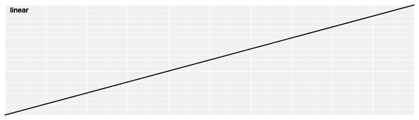 # d3.easePolyIn(t) <>
Polynomial easing; raises t to the specified exponent.
If the exponent is not specified, it defaults to 3, equivalent to cubicIn.
# d3.easePolyIn(t) <>
Polynomial easing; raises t to the specified exponent.
If the exponent is not specified, it defaults to 3, equivalent to cubicIn.
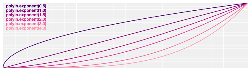 # d3.easePolyOut(t) <>
Reverse polynomial easing; equivalent to 1 - polyIn(1 - t).
If the exponent is not specified, it defaults to 3, equivalent to cubicOut.
# d3.easePolyOut(t) <>
Reverse polynomial easing; equivalent to 1 - polyIn(1 - t).
If the exponent is not specified, it defaults to 3, equivalent to cubicOut.
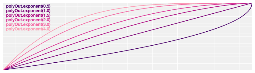 # d3.easePoly(t) <>
# d3.easePolyInOut(t) <>
Symmetric polynomial easing; scales polyIn for t in [0, 0.5] and polyOut for t in [0.5, 1].
If the exponent is not specified, it defaults to 3, equivalent to cubic.
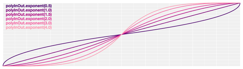 # poly.exponent(e) <>
Returns a new polynomial easing with the specified exponent e.
For example, to create equivalents of linear, quad, and cubic:
var linear = d3.easePoly.exponent(1),
quad = d3.easePoly.exponent(2),
cubic = d3.easePoly.exponent(3);
# d3.easeQuadIn(t) <>
Quadratic easing; equivalent to polyIn.exponent(2).
# poly.exponent(e) <>
Returns a new polynomial easing with the specified exponent e.
For example, to create equivalents of linear, quad, and cubic:
var linear = d3.easePoly.exponent(1),
quad = d3.easePoly.exponent(2),
cubic = d3.easePoly.exponent(3);
# d3.easeQuadIn(t) <>
Quadratic easing; equivalent to polyIn.exponent(2).
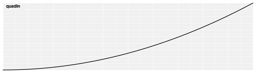 # d3.easeQuadOut(t) <>
Reverse quadratic easing; equivalent to 1 - quadIn(1 - t).
Also equivalent to polyOut.exponent(2).
# d3.easeQuadOut(t) <>
Reverse quadratic easing; equivalent to 1 - quadIn(1 - t).
Also equivalent to polyOut.exponent(2).
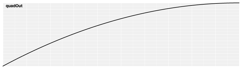 # d3.easeQuad(t) <>
# d3.easeQuadInOut(t) <>
Symmetric quadratic easing; scales quadIn for t in [0, 0.5] and quadOut for t in [0.5, 1].
Also equivalent to poly.exponent(2).
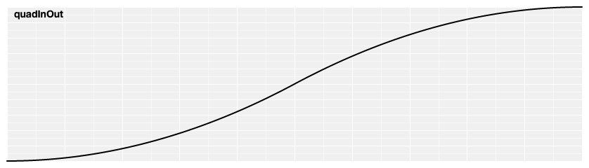 # d3.easeCubicIn(t) <>
Cubic easing; equivalent to polyIn.exponent(3).
# d3.easeCubicIn(t) <>
Cubic easing; equivalent to polyIn.exponent(3).
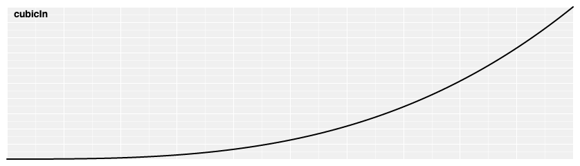 # d3.easeCubicOut(t) <>
Reverse cubic easing; equivalent to 1 - cubicIn(1 - t).
Also equivalent to polyOut.exponent(3).
# d3.easeCubicOut(t) <>
Reverse cubic easing; equivalent to 1 - cubicIn(1 - t).
Also equivalent to polyOut.exponent(3).
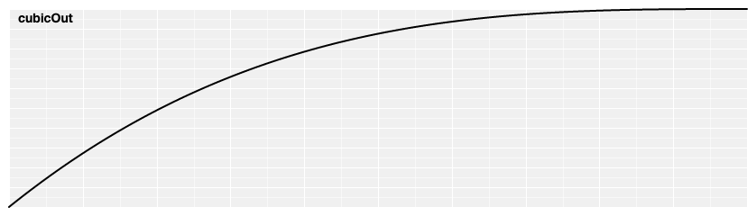 # d3.easeCubic(t) <>
# d3.easeCubicInOut(t) <>
Symmetric cubic easing; scales cubicIn for t in [0, 0.5] and cubicOut for t in [0.5, 1].
Also equivalent to poly.exponent(3).
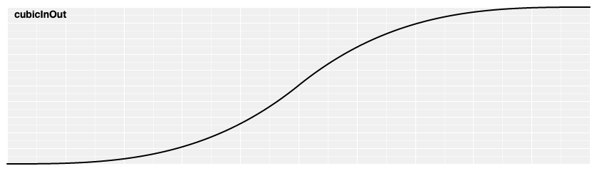 # d3.easeSinIn(t) <>
Sinusoidal easing; returns sin(t).
# d3.easeSinIn(t) <>
Sinusoidal easing; returns sin(t).
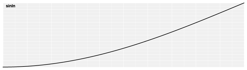 # d3.easeSinOut(t) <>
Reverse sinusoidal easing; equivalent to 1 - sinIn(1 - t).
# d3.easeSinOut(t) <>
Reverse sinusoidal easing; equivalent to 1 - sinIn(1 - t).
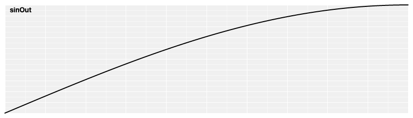 # d3.easeSin(t) <>
# d3.easeSinInOut(t) <>
Symmetric sinusoidal easing; scales sinIn for t in [0, 0.5] and sinOut for t in [0.5, 1].
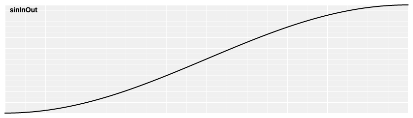 # d3.easeExpIn(t) <>
Exponential easing; raises 2 to the exponent 10 * (t - 1).
# d3.easeExpIn(t) <>
Exponential easing; raises 2 to the exponent 10 * (t - 1).
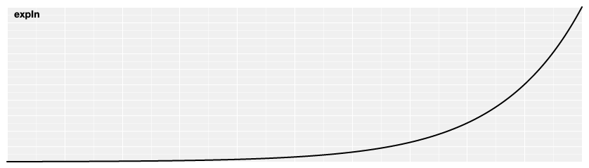 # d3.easeExpOut(t) <>
Reverse exponential easing; equivalent to 1 - expIn(1 - t).
# d3.easeExpOut(t) <>
Reverse exponential easing; equivalent to 1 - expIn(1 - t).
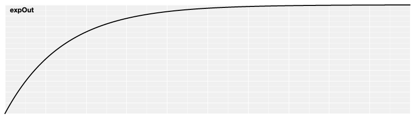 # d3.easeExp(t) <>
# d3.easeExpInOut(t) <>
Symmetric exponential easing; scales expIn for t in [0, 0.5] and expOut for t in [0.5, 1].
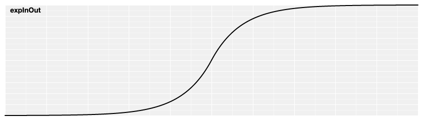 # d3.easeCircleIn(t) <>
Circular easing.
# d3.easeCircleIn(t) <>
Circular easing.
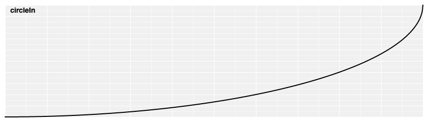 # d3.easeCircleOut(t) <>
Reverse circular easing; equivalent to 1 - circleIn(1 - t).
# d3.easeCircleOut(t) <>
Reverse circular easing; equivalent to 1 - circleIn(1 - t).
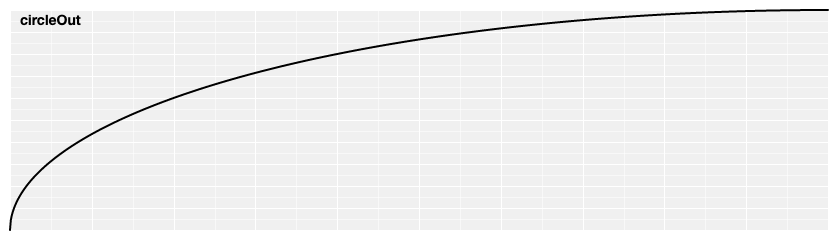 # d3.easeCircle(t) <>
# d3.easeCircleInOut(t) <>
Symmetric circular easing; scales circleIn for t in [0, 0.5] and circleOut for t in [0.5, 1].
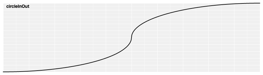 # d3.easeElasticIn(t) <>
Elastic easing, like a rubber band.
The amplitude and period of the oscillation are configurable; if not specified, they default to 1 and 0.3, respectively.
# d3.easeElasticIn(t) <>
Elastic easing, like a rubber band.
The amplitude and period of the oscillation are configurable; if not specified, they default to 1 and 0.3, respectively.
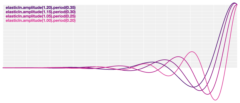 # d3.easeElastic(t) <>
# d3.easeElasticOut(t) <>
Reverse elastic easing; equivalent to 1 - elasticIn(1 - t).
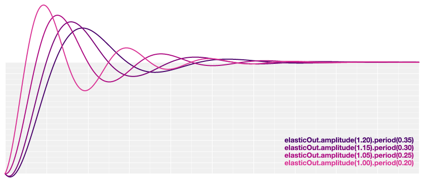 # d3.easeElasticInOut(t) <>
Symmetric elastic easing; scales elasticIn for t in [0, 0.5] and elasticOut for t in [0.5, 1].
# d3.easeElasticInOut(t) <>
Symmetric elastic easing; scales elasticIn for t in [0, 0.5] and elasticOut for t in [0.5, 1].
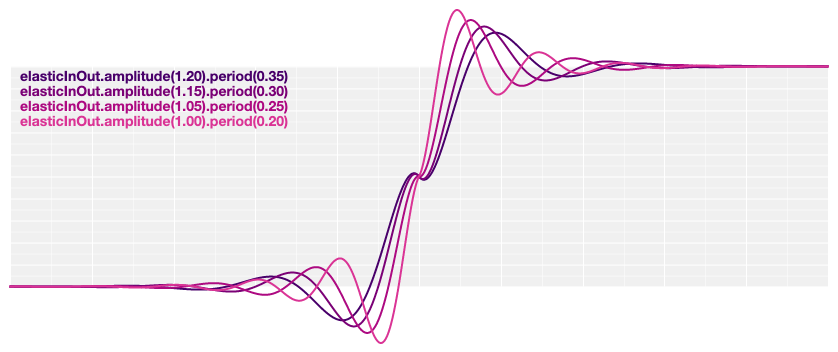 # elastic.amplitude(a) <>
Returns a new elastic easing with the specified amplitude a.
# elastic.period(p) <>
Returns a new elastic easing with the specified period p.
# d3.easeBackIn(t) <>
Anticipatory easing, like a dancer bending his knees before jumping off the floor.
The degree of overshoot is configurable; if not specified, it defaults to 1.70158.
# elastic.amplitude(a) <>
Returns a new elastic easing with the specified amplitude a.
# elastic.period(p) <>
Returns a new elastic easing with the specified period p.
# d3.easeBackIn(t) <>
Anticipatory easing, like a dancer bending his knees before jumping off the floor.
The degree of overshoot is configurable; if not specified, it defaults to 1.70158.
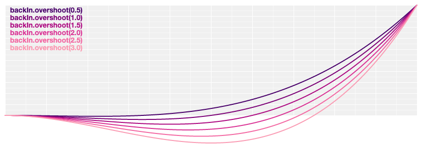 # d3.easeBackOut(t) <>
Reverse anticipatory easing; equivalent to 1 - backIn(1 - t).
# d3.easeBackOut(t) <>
Reverse anticipatory easing; equivalent to 1 - backIn(1 - t).
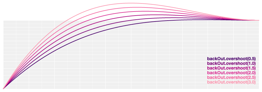 # d3.easeBack(t) <>
# d3.easeBackInOut(t) <>
Symmetric anticipatory easing; scales backIn for t in [0, 0.5] and backOut for t in [0.5, 1].
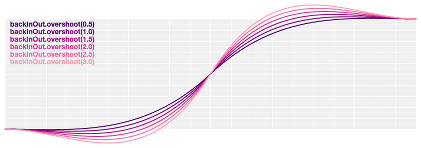 # back.overshoot(s) <>
Returns a new back easing with the specified overshoot s.
# d3.easeBounceIn(t) <>
Bounce easing, like a rubber ball.
# back.overshoot(s) <>
Returns a new back easing with the specified overshoot s.
# d3.easeBounceIn(t) <>
Bounce easing, like a rubber ball.
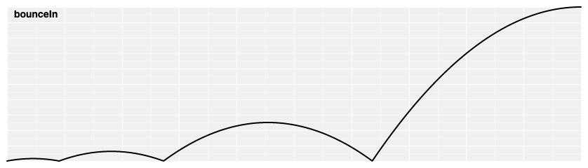 # d3.easeBounce(t) <>
# d3.easeBounceOut(t) <>
Reverse bounce easing; equivalent to 1 - bounceIn(1 - t).
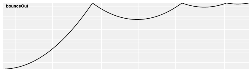 # d3.easeBounceInOut(t) <>
Symmetric bounce easing; scales bounceIn for t in [0, 0.5] and bounceOut for t in [0.5, 1].
# d3.easeBounceInOut(t) <>
Symmetric bounce easing; scales bounceIn for t in [0, 0.5] and bounceOut for t in [0.5, 1].
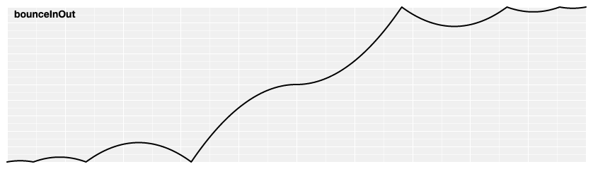
d3-fetch
This module provides convenient parsing on top of Fetch.
For example, to load a text file:
d3.text("/path/to/file.txt").then(function(text) {
console.log(text); // Hello, world!
});
To load and parse a CSV file:
d3.csv("/path/to/file.csv").then(function(data) {
console.log(data); // [{"Hello": "world"}, …]
});
This module has built-in support for parsing JSON, CSV, and TSV.
You can parse additional formats by using text directly.
(This module replaced d3-request.)
Installing
If you use NPM, npm install d3-fetch.
Otherwise, download the latest release.
You can also load directly from d3js.org as a standalone library.
AMD, CommonJS, and vanilla environments are supported.
In vanilla, a d3 global is exported:
<script src="https://d3js.org/d3-dsv.v2.min.js"></script>
<script src="https://d3js.org/d3-fetch.v2.min.js"></script>
<script>
d3.csv("/path/to/file.csv").then(function(data) {
console.log(data); // [{"Hello": "world"}, …]
});
</script>
API Reference
# d3.blob(input[, init]) <>
Fetches the binary file at the specified input URL as a Blob.
If init is specified, it is passed along to the underlying call to fetch; see RequestInit for allowed fields.
# d3.buffer(input[, init]) <>
Fetches the binary file at the specified input URL as an ArrayBuffer.
If init is specified, it is passed along to the underlying call to fetch; see RequestInit for allowed fields.
# d3.csv(input[, init][, row]) <>
Equivalent to d3.dsv with the comma character as the delimiter.
# d3.dsv(delimiter, input[, init][, row]) <>
Fetches the DSV file at the specified input URL.
If init is specified, it is passed along to the underlying call to fetch; see RequestInit for allowed fields.
An optional row conversion function may be specified to map and filter row objects to a more-specific representation; see dsv.parse for details.
For example:
d3.dsv(",", "test.csv", function(d) {
return {
year: new Date(+d.Year, 0, 1), // convert "Year" column to Date
make: d.Make,
model: d.Model,
length: +d.Length // convert "Length" column to number
};
}).then(function(data) {
console.log(data);
});
If only one of init and row is specified, it is interpreted as the row conversion function if it is a function, and otherwise an init object.
See also d3.csv and d3.tsv.
# d3.html(input[, init]) <>
Fetches the file at the specified input URL as text and then parses it as HTML.
If init is specified, it is passed along to the underlying call to fetch; see RequestInit for allowed fields.
# d3.image(input[, init]) <>
Fetches the image at the specified input URL.
If init is specified, sets any additional properties on the image before loading.
For example, to enable an anonymous cross-origin request:
d3.image("https://example.com/test.png", {crossOrigin: "anonymous"}).then(function(img) {
console.log(img);
});
# d3.json(input[, init]) <>
Fetches the JSON file at the specified input URL.
If init is specified, it is passed along to the underlying call to fetch; see RequestInit for allowed fields.
If the server returns a status code of 204 No Content or 205 Reset Content, the promise resolves to undefined.
# d3.svg(input[, init]) <>
Fetches the file at the specified input URL as text and then parses it as SVG.
If init is specified, it is passed along to the underlying call to fetch; see RequestInit for allowed fields.
# d3.text(input[, init]) <>
Fetches the text file at the specified input URL.
If init is specified, it is passed along to the underlying call to fetch; see RequestInit for allowed fields.
# d3.tsv(input[, init][, row]) <>
Equivalent to d3.dsv with the tab character as the delimiter.
# d3.xml(input[, init]) <>
Fetches the file at the specified input URL as text and then parses it as XML.
If init is specified, it is passed along to the underlying call to fetch; see RequestInit for allowed fields.
d3-force
This module implements a velocity Verlet numerical integrator for simulating physical forces on particles.
The simulation is simplified: it assumes a constant unit time step t = 1 for each step, and a constant unit mass m = 1 for all particles.
As a result, a force F acting on a particle is equivalent to a constant acceleration a over the time interval t, and can be simulated simply by adding to the particle’s velocity, which is then added to the particle’s position.
In the domain of information visualization, physical simulations are useful for studying networks and hierarchies!
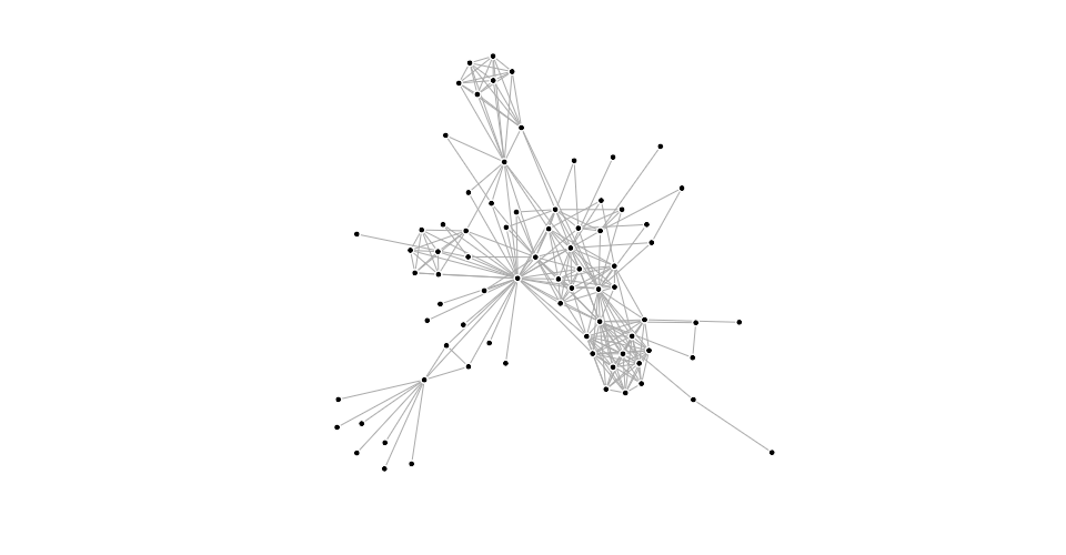
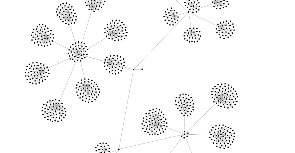 You can also simulate circles (disks) with collision, such as for bubble charts or beeswarm plots:
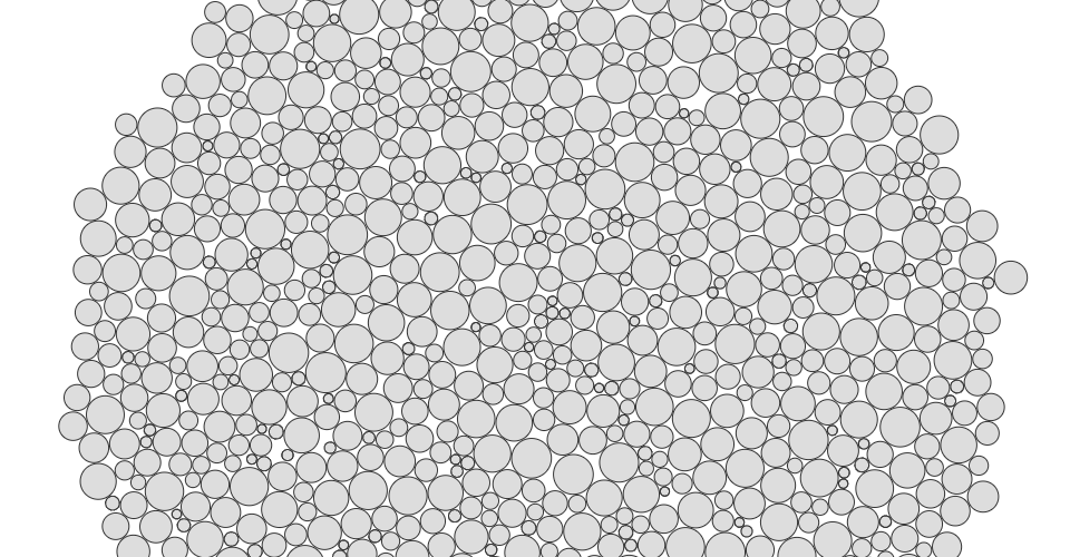
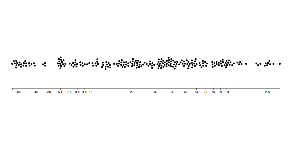 You can even use it as a rudimentary physics engine, say to simulate cloth:
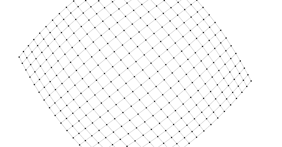 To use this module, create a simulation for an array of nodes, and compose the desired forces.
Then listen for tick events to render the nodes as they update in your preferred graphics system, such as Canvas or SVG.
To use this module, create a simulation for an array of nodes, and compose the desired forces.
Then listen for tick events to render the nodes as they update in your preferred graphics system, such as Canvas or SVG.
Installing
If you use NPM, npm install d3-force.
Otherwise, download the latest release.
You can also load directly from d3js.org, either as a standalone library or as part of D3.
AMD, CommonJS, and vanilla environments are supported.
In vanilla, a d3_force global is exported:
<script src="https://d3js.org/d3-dispatch.v1.min.js"></script>
<script src="https://d3js.org/d3-quadtree.v1.min.js"></script>
<script src="https://d3js.org/d3-timer.v1.min.js"></script>
<script src="https://d3js.org/d3-force.v2.min.js"></script>
<script>
var simulation = d3.forceSimulation(nodes);
</script>
Try d3-force in your browser.
API Reference
Simulation
# d3.forceSimulation([nodes]) <>
Creates a new simulation with the specified array of nodes and no forces.
If nodes is not specified, it defaults to the empty array.
The simulator starts automatically; use simulation.on to listen for tick events as the simulation runs.
If you wish to run the simulation manually instead, call simulation.stop, and then call simulation.tick as desired.
# simulation.restart() <>
Restarts the simulation’s internal timer and returns the simulation.
In conjunction with simulation.alphaTarget or simulation.alpha, this method can be used to “reheat” the simulation during interaction, such as when dragging a node, or to resume the simulation after temporarily pausing it with simulation.stop.
# simulation.stop() <>
Stops the simulation’s internal timer, if it is running, and returns the simulation.
If the timer is already stopped, this method does nothing.
This method is useful for running the simulation manually; see simulation.tick.
# simulation.tick([iterations]) <>
Manually steps the simulation by the specified number of iterations, and returns the simulation.
If iterations is not specified, it defaults to 1 (single step).
For each iteration, it increments the current alpha by (alphaTarget - alpha) × alphaDecay; then invokes each registered force, passing the new alpha; then decrements each node’s velocity by velocity × velocityDecay; lastly increments each node’s position by velocity.
This method does not dispatch events; events are only dispatched by the internal timer when the simulation is started automatically upon creation or by calling simulation.restart.
The natural number of ticks when the simulation is started is log(alphaMin) / log(1 - alphaDecay); by default, this is 300.
This method can be used in conjunction with simulation.stop to compute a static force layout.
For large graphs, static layouts should be computed in a web worker to avoid freezing the user interface.
# simulation.nodes([nodes]) <>
If nodes is specified, sets the simulation’s nodes to the specified array of objects, initializing their positions and velocities if necessary, and then re-initializes any bound forces; returns the simulation.
If nodes is not specified, returns the simulation’s array of nodes as specified to the constructor.
Each node must be an object.
The following properties are assigned by the simulation:
index - the node’s zero-based index into nodes
x - the node’s current x-position
y - the node’s current y-position
vx - the node’s current x-velocity
vy - the node’s current y-velocity
The position x,y and velocity vx,vy may be subsequently modified by forces and by the simulation.
If either vx or vy is NaN, the velocity is initialized to 0,0.
If either x or y is NaN, the position is initialized in a phyllotaxis arrangement, so chosen to ensure a deterministic, uniform distribution.
To fix a node in a given position, you may specify two additional properties:
fx - the node’s fixed x-position
fy - the node’s fixed y-position
At the end of each tick, after the application of any forces, a node with a defined node.fx has node.x reset to this value and node.vx set to zero; likewise, a node with a defined node.fy has node.y reset to this value and node.vy set to zero.
To unfix a node that was previously fixed, set node.fx and node.fy to null, or delete these properties.
If the specified array of nodes is modified, such as when nodes are added to or removed from the simulation, this method must be called again with the new (or changed) array to notify the simulation and bound forces of the change; the simulation does not make a defensive copy of the specified array.
# simulation.alpha([alpha]) <>
alpha is roughly analogous to temperature in simulated annealing.
It decreases over time as the simulation “cools down”.
When alpha reaches alphaMin, the simulation stops; see simulation.restart.
If alpha is specified, sets the current alpha to the specified number in the range [0,1] and returns this simulation.
If alpha is not specified, returns the current alpha value, which defaults to 1.
# simulation.alphaMin([min]) <>
If min is specified, sets the minimum alpha to the specified number in the range [0,1] and returns this simulation.
If min is not specified, returns the current minimum alpha value, which defaults to 0.001.
The simulation’s internal timer stops when the current alpha is less than the minimum alpha.
The default alpha decay rate of ~0.0228 corresponds to 300 iterations.
# simulation.alphaDecay([decay]) <>
If decay is specified, sets the alpha decay rate to the specified number in the range [0,1] and returns this simulation.
If decay is not specified, returns the current alpha decay rate, which defaults to 0.0228… = 1 - pow(0.001, 1 / 300) where 0.001 is the default minimum alpha.
The alpha decay rate determines how quickly the current alpha interpolates towards the desired target alpha; since the default target alpha is zero, by default this controls how quickly the simulation cools.
Higher decay rates cause the simulation to stabilize more quickly, but risk getting stuck in a local minimum; lower values cause the simulation to take longer to run, but typically converge on a better layout.
To have the simulation run forever at the current alpha, set the decay rate to zero; alternatively, set a target alpha greater than the minimum alpha.
# simulation.alphaTarget([target]) <>
If target is specified, sets the current target alpha to the specified number in the range [0,1] and returns this simulation.
If target is not specified, returns the current target alpha value, which defaults to 0.
# simulation.velocityDecay([decay]) <>
If decay is specified, sets the velocity decay factor to the specified number in the range [0,1] and returns this simulation.
If decay is not specified, returns the current velocity decay factor, which defaults to 0.4.
The decay factor is akin to atmospheric friction; after the application of any forces during a tick, each node’s velocity is multiplied by 1 - decay.
As with lowering the alpha decay rate, less velocity decay may converge on a better solution, but risks numerical instabilities and oscillation.
# simulation.force(name[, force]) <>
If force is specified, assigns the force for the specified name and returns this simulation.
If force is not specified, returns the force with the specified name, or undefined if there is no such force.
(By default, new simulations have no forces.) For example, to create a new simulation to layout a graph, you might say:
var simulation = d3.forceSimulation(nodes)
.force("charge", d3.forceManyBody())
.force("link", d3.forceLink(links))
.force("center", d3.forceCenter());
To remove the force with the given name, pass null as the force.
For example, to remove the charge force:
simulation.force("charge", null);
# simulation.find(x, y[, radius]) <>
Returns the node closest to the position x,y with the given search radius.
If radius is not specified, it defaults to infinity.
If there is no node within the search area, returns undefined.
# simulation.randomSource([source]) <>)
If source is specified, sets the function used to generate random numbers; this should be a function that returns a number between 0 (inclusive) and 1 (exclusive).
If source is not specified, returns this simulation’s current random source which defaults to a fixed-seed linear congruential generator.
See also random.source.
# simulation.on(typenames, [listener]) <>
If listener is specified, sets the event listener for the specified typenames and returns this simulation.
If an event listener was already registered for the same type and name, the existing listener is removed before the new listener is added.
If listener is null, removes the current event listeners for the specified typenames, if any.
If listener is not specified, returns the first currently-assigned listener matching the specified typenames, if any.
When a specified event is dispatched, each listener will be invoked with the this context as the simulation.
The typenames is a string containing one or more typename separated by whitespace.
Each typename is a type, optionally followed by a period (.) and a name, such as tick.foo and tick.bar; the name allows multiple listeners to be registered for the same type.
The type must be one of the following:
tick - after each tick of the simulation’s internal timer.
end - after the simulation’s timer stops when alpha < alphaMin.
Note that tick events are not dispatched when simulation.tick is called manually; events are only dispatched by the internal timer and are intended for interactive rendering of the simulation.
To affect the simulation, register forces instead of modifying nodes’ positions or velocities inside a tick event listener.
See dispatch.on for details.
Forces
A force is simply a function that modifies nodes’ positions or velocities; in this context, a force can apply a classical physical force such as electrical charge or gravity, or it can resolve a geometric constraint, such as keeping nodes within a bounding box or keeping linked nodes a fixed distance apart.
For example, a simple positioning force that moves nodes towards the origin 0,0 might be implemented as:
function force(alpha) {
for (var i = 0, n = nodes.length, node, k = alpha * 0.1; i < n; ++i) {
node = nodes[i];
node.vx -= node.x * k;
node.vy -= node.y * k;
}
}
Forces typically read the node’s current position x,y and then add to (or subtract from) the node’s velocity vx,vy.
However, forces may also “peek ahead” to the anticipated next position of the node, x + vx,y + vy; this is necessary for resolving geometric constraints through iterative relaxation.
Forces may also modify the position directly, which is sometimes useful to avoid adding energy to the simulation, such as when recentering the simulation in the viewport.
Simulations typically compose multiple forces as desired.
This module provides several for your enjoyment:
Centering
Collision
Links
Many-Body
Positioning
Forces may optionally implement force.initialize to receive the simulation’s array of nodes.
# force(alpha) <>
Applies this force, optionally observing the specified alpha.
Typically, the force is applied to the array of nodes previously passed to force.initialize, however, some forces may apply to a subset of nodes, or behave differently.
For example, d3.forceLink applies to the source and target of each link.
# force.initialize(nodes, random) <>
Supplies the array of nodes and random source to this force.
This method is called when a force is bound to a simulation via simulation.force and when the simulation’s nodes change via simulation.nodes.
A force may perform necessary work during initialization, such as evaluating per-node parameters, to avoid repeatedly performing work during each application of the force.
Centering
The centering force translates nodes uniformly so that the mean position of all nodes (the center of mass if all nodes have equal weight) is at the given position x,y.
This force modifies the positions of nodes on each application; it does not modify velocities, as doing so would typically cause the nodes to overshoot and oscillate around the desired center.
This force helps keeps nodes in the center of the viewport, and unlike the positioning force, it does not distort their relative positions.
# d3.forceCenter([x, y]) <>
Creates a new centering force with the specified x- and y- coordinates.
If x and y are not specified, they default to 0,0.
# center.x([x]) <>
If x is specified, sets the x-coordinate of the centering position to the specified number and returns this force.
If x is not specified, returns the current x-coordinate, which defaults to zero.
# center.y([y]) <>
If y is specified, sets the y-coordinate of the centering position to the specified number and returns this force.
If y is not specified, returns the current y-coordinate, which defaults to zero.
# center.strength([strength]) · <>
If strength is specified, sets the centering force’s strength.
A reduced strength of e.g.
0.05 softens the movements on interactive graphs in which new nodes enter or exit the graph.
If strength is not specified, returns the force’s current strength, which defaults to 1.
Collision
The collision force treats nodes as circles with a given radius, rather than points, and prevents nodes from overlapping.
More formally, two nodes a and b are separated so that the distance between a and b is at least radius(a) + radius(b).
To reduce jitter, this is by default a “soft” constraint with a configurable strength and iteration count.
# d3.forceCollide([radius]) <>
Creates a new circle collision force with the specified radius.
If radius is not specified, it defaults to the constant one for all nodes.
# collide.radius([radius]) <>
If radius is specified, sets the radius accessor to the specified number or function, re-evaluates the radius accessor for each node, and returns this force.
If radius is not specified, returns the current radius accessor, which defaults to:
function radius() {
return 1;
}
The radius accessor is invoked for each node in the simulation, being passed the node and its zero-based index.
The resulting number is then stored internally, such that the radius of each node is only recomputed when the force is initialized or when this method is called with a new radius, and not on every application of the force.
# collide.strength([strength]) <>
If strength is specified, sets the force strength to the specified number in the range [0,1] and returns this force.
If strength is not specified, returns the current strength which defaults to 1.
Overlapping nodes are resolved through iterative relaxation.
For each node, the other nodes that are anticipated to overlap at the next tick (using the anticipated positions x + vx,y + vy) are determined; the node’s velocity is then modified to push the node out of each overlapping node.
The change in velocity is dampened by the force’s strength such that the resolution of simultaneous overlaps can be blended together to find a stable solution.
# collide.iterations([iterations]) <>
If iterations is specified, sets the number of iterations per application to the specified number and returns this force.
If iterations is not specified, returns the current iteration count which defaults to 1.
Increasing the number of iterations greatly increases the rigidity of the constraint and avoids partial overlap of nodes, but also increases the runtime cost to evaluate the force.
Links
The link force pushes linked nodes together or apart according to the desired link distance.
The strength of the force is proportional to the difference between the linked nodes’ distance and the target distance, similar to a spring force.
# d3.forceLink([links]) <>
Creates a new link force with the specified links and default parameters.
If links is not specified, it defaults to the empty array.
# link.links([links]) <>
If links is specified, sets the array of links associated with this force, recomputes the distance and strength parameters for each link, and returns this force.
If links is not specified, returns the current array of links, which defaults to the empty array.
Each link is an object with the following properties:
source - the link’s source node; see simulation.nodes
target - the link’s target node; see simulation.nodes
index - the zero-based index into links, assigned by this method
For convenience, a link’s source and target properties may be initialized using numeric or string identifiers rather than object references; see link.id.
When the link force is initialized (or re-initialized, as when the nodes or links change), any link.source or link.target property which is not an object is replaced by an object reference to the corresponding node with the given identifier.
If the specified array of links is modified, such as when links are added to or removed from the simulation, this method must be called again with the new (or changed) array to notify the force of the change; the force does not make a defensive copy of the specified array.
# link.id([id]) <>
If id is specified, sets the node id accessor to the specified function and returns this force.
If id is not specified, returns the current node id accessor, which defaults to the numeric node.index:
function id(d) {
return d.index;
}
The default id accessor allows each link’s source and target to be specified as a zero-based index into the nodes array.
For example:
var nodes = [
{"id": "Alice"},
{"id": "Bob"},
{"id": "Carol"}
];
var links = [
{"source": 0, "target": 1}, // Alice Bob
{"source": 1, "target": 2} // Bob Carol
];
Now consider a different id accessor that returns a string:
function id(d) {
return d.id;
}
With this accessor, you can use named sources and targets:
var nodes = [
{"id": "Alice"},
{"id": "Bob"},
{"id": "Carol"}
];
var links = [
{"source": "Alice", "target": "Bob"},
{"source": "Bob", "target": "Carol"}
];
This is particularly useful when representing graphs in JSON, as JSON does not allow references.
See this example.
The id accessor is invoked for each node whenever the force is initialized, as when the nodes or links change, being passed the node and its zero-based index.
# link.distance([distance]) <>
If distance is specified, sets the distance accessor to the specified number or function, re-evaluates the distance accessor for each link, and returns this force.
If distance is not specified, returns the current distance accessor, which defaults to:
function distance() {
return 30;
}
The distance accessor is invoked for each link, being passed the link and its zero-based index.
The resulting number is then stored internally, such that the distance of each link is only recomputed when the force is initialized or when this method is called with a new distance, and not on every application of the force.
# link.strength([strength]) <>
If strength is specified, sets the strength accessor to the specified number or function, re-evaluates the strength accessor for each link, and returns this force.
If strength is not specified, returns the current strength accessor, which defaults to:
function strength(link) {
return 1 / Math.min(count(link.source), count(link.target));
}
Where count(node) is a function that returns the number of links with the given node as a source or target.
This default was chosen because it automatically reduces the strength of links connected to heavily-connected nodes, improving stability.
The strength accessor is invoked for each link, being passed the link and its zero-based index.
The resulting number is then stored internally, such that the strength of each link is only recomputed when the force is initialized or when this method is called with a new strength, and not on every application of the force.
# link.iterations([iterations]) <>
If iterations is specified, sets the number of iterations per application to the specified number and returns this force.
If iterations is not specified, returns the current iteration count which defaults to 1.
Increasing the number of iterations greatly increases the rigidity of the constraint and is useful for complex structures such as lattices, but also increases the runtime cost to evaluate the force.
Many-Body
The many-body (or n-body) force applies mutually amongst all nodes.
It can be used to simulate gravity (attraction) if the strength is positive, or electrostatic charge (repulsion) if the strength is negative.
This implementation uses quadtrees and the Barnes–Hut approximation to greatly improve performance; the accuracy can be customized using the theta parameter.
Unlike links, which only affect two linked nodes, the charge force is global: every node affects every other node, even if they are on disconnected subgraphs.
# d3.forceManyBody() <>
Creates a new many-body force with the default parameters.
# manyBody.strength([strength]) <>
If strength is specified, sets the strength accessor to the specified number or function, re-evaluates the strength accessor for each node, and returns this force.
A positive value causes nodes to attract each other, similar to gravity, while a negative value causes nodes to repel each other, similar to electrostatic charge.
If strength is not specified, returns the current strength accessor, which defaults to:
function strength() {
return -30;
}
The strength accessor is invoked for each node in the simulation, being passed the node and its zero-based index.
The resulting number is then stored internally, such that the strength of each node is only recomputed when the force is initialized or when this method is called with a new strength, and not on every application of the force.
# manyBody.theta([theta]) <>
If theta is specified, sets the Barnes–Hut approximation criterion to the specified number and returns this force.
If theta is not specified, returns the current value, which defaults to 0.9.
To accelerate computation, this force implements the Barnes–Hut approximation which takes O(n log n) per application where n is the number of nodes.
For each application, a quadtree stores the current node positions; then for each node, the combined force of all other nodes on the given node is computed.
For a cluster of nodes that is far away, the charge force can be approximated by treating the cluster as a single, larger node.
The theta parameter determines the accuracy of the approximation: if the ratio w / l of the width w of the quadtree cell to the distance l from the node to the cell’s center of mass is less than theta, all nodes in the given cell are treated as a single node rather than individually.
# manyBody.distanceMin([distance]) <>
If distance is specified, sets the minimum distance between nodes over which this force is considered.
If distance is not specified, returns the current minimum distance, which defaults to 1.
A minimum distance establishes an upper bound on the strength of the force between two nearby nodes, avoiding instability.
In particular, it avoids an infinitely-strong force if two nodes are exactly coincident; in this case, the direction of the force is random.
# manyBody.distanceMax([distance]) <>
If distance is specified, sets the maximum distance between nodes over which this force is considered.
If distance is not specified, returns the current maximum distance, which defaults to infinity.
Specifying a finite maximum distance improves performance and produces a more localized layout.
Positioning
The x- and y-positioning forces push nodes towards a desired position along the given dimension with a configurable strength.
The radial force is similar, except it pushes nodes towards the closest point on a given circle.
The strength of the force is proportional to the one-dimensional distance between the node’s position and the target position.
While these forces can be used to position individual nodes, they are intended primarily for global forces that apply to all (or most) nodes.
# d3.forceX([x]) <>
Creates a new positioning force along the x-axis towards the given position x.
If x is not specified, it defaults to 0.
# x.strength([strength]) <>
If strength is specified, sets the strength accessor to the specified number or function, re-evaluates the strength accessor for each node, and returns this force.
The strength determines how much to increment the node’s x-velocity: (x - node.x) × strength.
For example, a value of 0.1 indicates that the node should move a tenth of the way from its current x-position to the target x-position with each application.
Higher values moves nodes more quickly to the target position, often at the expense of other forces or constraints.
A value outside the range [0,1] is not recommended.
If strength is not specified, returns the current strength accessor, which defaults to:
function strength() {
return 0.1;
}
The strength accessor is invoked for each node in the simulation, being passed the node and its zero-based index.
The resulting number is then stored internally, such that the strength of each node is only recomputed when the force is initialized or when this method is called with a new strength, and not on every application of the force.
# x.x([x]) <>
If x is specified, sets the x-coordinate accessor to the specified number or function, re-evaluates the x-accessor for each node, and returns this force.
If x is not specified, returns the current x-accessor, which defaults to:
function x() {
return 0;
}
The x-accessor is invoked for each node in the simulation, being passed the node and its zero-based index.
The resulting number is then stored internally, such that the target x-coordinate of each node is only recomputed when the force is initialized or when this method is called with a new x, and not on every application of the force.
# d3.forceY([y]) <>
Creates a new positioning force along the y-axis towards the given position y.
If y is not specified, it defaults to 0.
# y.strength([strength]) <>
If strength is specified, sets the strength accessor to the specified number or function, re-evaluates the strength accessor for each node, and returns this force.
The strength determines how much to increment the node’s y-velocity: (y - node.y) × strength.
For example, a value of 0.1 indicates that the node should move a tenth of the way from its current y-position to the target y-position with each application.
Higher values moves nodes more quickly to the target position, often at the expense of other forces or constraints.
A value outside the range [0,1] is not recommended.
If strength is not specified, returns the current strength accessor, which defaults to:
function strength() {
return 0.1;
}
The strength accessor is invoked for each node in the simulation, being passed the node and its zero-based index.
The resulting number is then stored internally, such that the strength of each node is only recomputed when the force is initialized or when this method is called with a new strength, and not on every application of the force.
# y.y([y]) <>
If y is specified, sets the y-coordinate accessor to the specified number or function, re-evaluates the y-accessor for each node, and returns this force.
If y is not specified, returns the current y-accessor, which defaults to:
function y() {
return 0;
}
The y-accessor is invoked for each node in the simulation, being passed the node and its zero-based index.
The resulting number is then stored internally, such that the target y-coordinate of each node is only recomputed when the force is initialized or when this method is called with a new y, and not on every application of the force.
# d3.forceRadial(radius[, x][, y]) <>
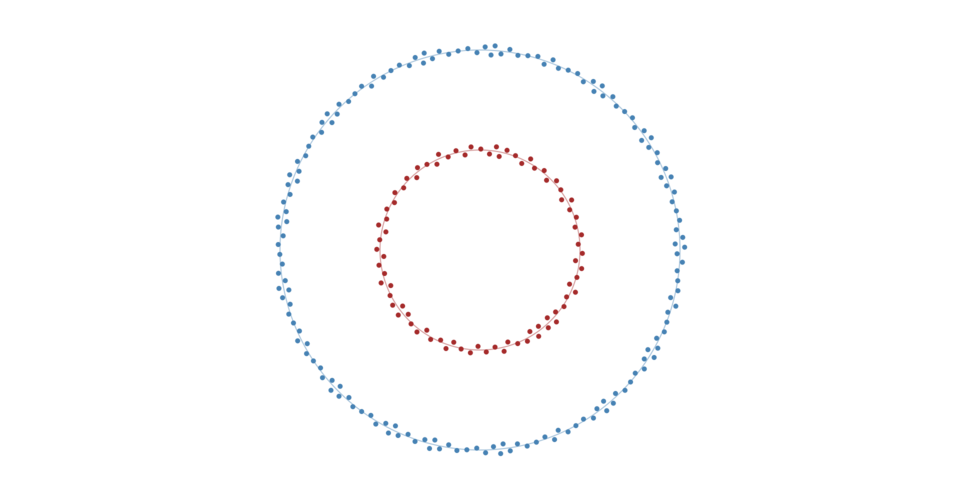 Creates a new positioning force towards a circle of the specified radius centered at x,y.
If x and y are not specified, they default to 0,0.
# radial.strength([strength]) <>
If strength is specified, sets the strength accessor to the specified number or function, re-evaluates the strength accessor for each node, and returns this force.
The strength determines how much to increment the node’s x- and y-velocity.
For example, a value of 0.1 indicates that the node should move a tenth of the way from its current position to the closest point on the circle with each application.
Higher values moves nodes more quickly to the target position, often at the expense of other forces or constraints.
A value outside the range [0,1] is not recommended.
If strength is not specified, returns the current strength accessor, which defaults to:
function strength() {
return 0.1;
}
The strength accessor is invoked for each node in the simulation, being passed the node and its zero-based index.
The resulting number is then stored internally, such that the strength of each node is only recomputed when the force is initialized or when this method is called with a new strength, and not on every application of the force.
# radial.radius([radius]) <>
If radius is specified, sets the circle radius to the specified number or function, re-evaluates the radius accessor for each node, and returns this force.
If radius is not specified, returns the current radius accessor.
The radius accessor is invoked for each node in the simulation, being passed the node and its zero-based index.
The resulting number is then stored internally, such that the target radius of each node is only recomputed when the force is initialized or when this method is called with a new radius, and not on every application of the force.
# radial.x([x]) <>
If x is specified, sets the x-coordinate of the circle center to the specified number and returns this force.
If x is not specified, returns the current x-coordinate of the center, which defaults to zero.
# radial.y([y]) <>
If y is specified, sets the y-coordinate of the circle center to the specified number and returns this force.
If y is not specified, returns the current y-coordinate of the center, which defaults to zero.
Creates a new positioning force towards a circle of the specified radius centered at x,y.
If x and y are not specified, they default to 0,0.
# radial.strength([strength]) <>
If strength is specified, sets the strength accessor to the specified number or function, re-evaluates the strength accessor for each node, and returns this force.
The strength determines how much to increment the node’s x- and y-velocity.
For example, a value of 0.1 indicates that the node should move a tenth of the way from its current position to the closest point on the circle with each application.
Higher values moves nodes more quickly to the target position, often at the expense of other forces or constraints.
A value outside the range [0,1] is not recommended.
If strength is not specified, returns the current strength accessor, which defaults to:
function strength() {
return 0.1;
}
The strength accessor is invoked for each node in the simulation, being passed the node and its zero-based index.
The resulting number is then stored internally, such that the strength of each node is only recomputed when the force is initialized or when this method is called with a new strength, and not on every application of the force.
# radial.radius([radius]) <>
If radius is specified, sets the circle radius to the specified number or function, re-evaluates the radius accessor for each node, and returns this force.
If radius is not specified, returns the current radius accessor.
The radius accessor is invoked for each node in the simulation, being passed the node and its zero-based index.
The resulting number is then stored internally, such that the target radius of each node is only recomputed when the force is initialized or when this method is called with a new radius, and not on every application of the force.
# radial.x([x]) <>
If x is specified, sets the x-coordinate of the circle center to the specified number and returns this force.
If x is not specified, returns the current x-coordinate of the center, which defaults to zero.
# radial.y([y]) <>
If y is specified, sets the y-coordinate of the circle center to the specified number and returns this force.
If y is not specified, returns the current y-coordinate of the center, which defaults to zero.
d3-format
Ever noticed how sometimes JavaScript doesn’t display numbers the way you expect? Like, you tried to print tenths with a simple loop:
for (var i = 0; i < 10; i++) {
console.log(0.1 * i);
}
And you got this:
0
0.1
0.2
0.30000000000000004
0.4
0.5
0.6000000000000001
0.7000000000000001
0.8
0.9
Welcome to binary floating point! _
Yet rounding error is not the only reason to customize number formatting.
A table of numbers should be formatted consistently for comparison; above, 0.0 would be better than 0.
Large numbers should have grouped digits (e.g., 42,000) or be in scientific or metric notation (4.2e+4, 42k).
Currencies should have fixed precision ($3.50).
Reported numerical results should be rounded to significant digits (4021 becomes 4000).
Number formats should appropriate to the reader’s locale (42.000,00 or 42,000.00).
The list goes on.
Formatting numbers for human consumption is the purpose of d3-format, which is modeled after Python 3’s format specification mini-language (PEP 3101).
Revisiting the example above:
var f = d3.format(".1f");
for (var i = 0; i < 10; i++) {
console.log(f(0.1 * i));
}
Now you get this:
0.0
0.1
0.2
0.3
0.4
0.5
0.6
0.7
0.8
0.9
But d3-format is much more than an alias for number.toFixed! A few more examples:
d3.format(".0%")(0.123); // rounded percentage, "12%"
d3.format("($.2f")(-3.5); // localized fixed-point currency, "(£3.50)"
d3.format("+20")(42); // space-filled and signed, " +42"
d3.format(".^20")(42); // dot-filled and centered, ".........42........."
d3.format(".2s")(42e6); // SI-prefix with two significant digits, "42M"
d3.format("#x")(48879); // prefixed lowercase hexadecimal, "0xbeef"
d3.format(",.2r")(4223); // grouped thousands with two significant digits, "4,200"
See locale.format for a detailed specification, and try running d3.formatSpecifier on the above formats to decode their meaning.
Installing
If you use NPM, npm install d3-format.
Otherwise, download the latest release.
You can also load directly from d3js.org, either as a standalone library or as part of D3.
AMD, CommonJS, and vanilla environments are supported.
In vanilla, a d3 global is exported:
<script src="https://d3js.org/d3-format.v2.min.js"></script>
<script>
var format = d3.format(".2s");
</script>
Locale files are published to npm and can be loaded using d3.json.
For example, to set Russian as the default locale:
d3.json("https://cdn.jsdelivr.net/npm/d3-format@2/locale/ru-RU.json", function(error, locale) {
if (error) throw error;
d3.formatDefaultLocale(locale);
var format = d3.format("$,");
console.log(format(1234.56)); // 1 234,56 .
});
Try d3-format in your browser.
API Reference
# d3.format(specifier) <>
An alias for locale.format on the default locale.
# d3.formatPrefix(specifier, value) <>
An alias for locale.formatPrefix on the default locale.
# locale.format(specifier) <>
Returns a new format function for the given string specifier.
The returned function takes a number as the only argument, and returns a string representing the formatted number.
The general form of a specifier is:
[[fill]align][sign][symbol][0][width][,][.precision][~][type]
The fill can be any character.
The presence of a fill character is signaled by the align character following it, which must be one of the following:
> - Forces the field to be right-aligned within the available space.
(Default behavior).
< - Forces the field to be left-aligned within the available space.
^ - Forces the field to be centered within the available space.
= - like >, but with any sign and symbol to the left of any padding.
The sign can be:
- - nothing for zero or positive and a minus sign for negative.
(Default behavior.)
+ - a plus sign for zero or positive and a minus sign for negative.
( - nothing for zero or positive and parentheses for negative.
(space) - a space for zero or positive and a minus sign for negative.
The symbol can be:
$ - apply currency symbols per the locale definition.
# - for binary, octal, or hexadecimal notation, prefix by 0b, 0o, or 0x, respectively.
The zero (0) option enables zero-padding; this implicitly sets fill to 0 and align to =.
The width defines the minimum field width; if not specified, then the width will be determined by the content.
The comma (,) option enables the use of a group separator, such as a comma for thousands.
Depending on the type, the precision either indicates the number of digits that follow the decimal point (types f and %), or the number of significant digits (types e, g, r, s and p).
If the precision is not specified, it defaults to 6 for all types except b, o, d, x, X and c).
See precisionFixed and precisionRound for help picking an appropriate precision.
The ~ option trims insignificant trailing zeros across all format types.
This is most commonly used in conjunction with types r, e, s and %.
For example:
d3.format("s")(1500); // "1.50000k"
d3.format("~s")(1500); // "1.5k"
The available type values are:
e - exponent notation.
f - fixed point notation.
g - either decimal or exponent notation, rounded to significant digits.
r - decimal notation, rounded to significant digits.
s - decimal notation with an SI prefix, rounded to significant digits.
% - multiply by 100, and then decimal notation with a percent sign.
p - multiply by 100, round to significant digits, and then decimal notation with a percent sign.
b - binary notation, rounded to integer.
o - octal notation, rounded to integer.
d - decimal notation, rounded to integer.
x - hexadecimal notation, using lower-case letters, rounded to integer.
X - hexadecimal notation, using upper-case letters, rounded to integer.
c - converts the integer to the corresponding unicode character before printing.
The type ~g (with a default precision of 12 instead of 6), and the type n is shorthand for ,g.
For the g, n and y - yocto, 10²4
z - zepto, 10²¹
a - atto, 10¹8
f - femto, 10¹5
p - pico, 10¹²
n - nano, 10
µ - micro, 106
m - milli, 10³
k - kilo, 10³
M - mega, 106
G - giga, 10
T - tera, 10¹²
P - peta, 10¹5
E - exa, 10¹8
Z - zetta, 10²¹
Y - yotta, 10²4
Unlike locale.format with the s format type, this method returns a formatter with a consistent SI prefix, rather than computing the prefix dynamically for each number.
In addition, the precision for the given specifier represents the number of digits past the decimal point (as with f fixed point notation), not the number of significant digits.
For example:
var f = d3.formatPrefix(",.0", 1e-6);
f(0.00042); // "420µ"
f(0.0042); // "4,200µ"
This method is useful when formatting multiple numbers in the same units for easy comparison.
See precisionPrefix for help picking an appropriate precision, and bl.ocks.org/9764126 for an example.
# d3.formatSpecifier(specifier) <>
Parses the specified specifier, returning an object with exposed fields that correspond to the format specification mini-language and a toString method that reconstructs the specifier.
For example, formatSpecifier("s") returns:
FormatSpecifier {
"fill": " ",
"align": ">",
"sign": "-",
"symbol": "",
"zero": false,
"width": undefined,
"comma": false,
"precision": undefined,
"trim": false,
"type": "s"
}
This method is useful for understanding how format specifiers are parsed and for deriving new specifiers.
For example, you might compute an appropriate precision based on the numbers you want to format using precisionFixed and then create a new format:
var s = d3.formatSpecifier("f");
s.precision = d3.precisionFixed(0.01);
var f = d3.format(s);
f(42); // "42.00";
# new d3.FormatSpecifier(specifier) <>
Given the specified specifier object, returning an object with exposed fields that correspond to the format specification mini-language and a toString method that reconstructs the specifier.
For example, new FormatSpecifier({type: "s"}) returns:
FormatSpecifier {
"fill": " ",
"align": ">",
"sign": "-",
"symbol": "",
"zero": false,
"width": undefined,
"comma": false,
"precision": undefined,
"trim": false,
"type": "s"
}
# d3.precisionFixed(step) <>
Returns a suggested decimal precision for fixed point notation given the specified numeric step value.
The step represents the minimum absolute difference between values that will be formatted.
(This assumes that the values to be formatted are also multiples of step.) For example, given the numbers 1, 1.5, and 2, the step should be 0.5 and the suggested precision is 1:
var p = d3.precisionFixed(0.5),
f = d3.format("." + p + "f");
f(1); // "1.0"
f(1.5); // "1.5"
f(2); // "2.0"
Whereas for the numbers 1, 2 and 3, the step should be 1 and the suggested precision is 0:
var p = d3.precisionFixed(1),
f = d3.format("." + p + "f");
f(1); // "1"
f(2); // "2"
f(3); // "3"
Note: for the % format type, subtract two:
var p = Math.max(0, d3.precisionFixed(0.05) - 2),
f = d3.format("." + p + "%");
f(0.45); // "45%"
f(0.50); // "50%"
f(0.55); // "55%"
# d3.precisionPrefix(step, value) <>
Returns a suggested decimal precision for use with locale.formatPrefix given the specified numeric step and reference value.
The step represents the minimum absolute difference between values that will be formatted, and value determines which SI prefix will be used.
(This assumes that the values to be formatted are also multiples of step.) For example, given the numbers 1.1e6, 1.2e6, and 1.3e6, the step should be 1e5, the value could be 1.3e6, and the suggested precision is 1:
var p = d3.precisionPrefix(1e5, 1.3e6),
f = d3.formatPrefix("." + p, 1.3e6);
f(1.1e6); // "1.1M"
f(1.2e6); // "1.2M"
f(1.3e6); // "1.3M"
# d3.precisionRound(step, max) <>
Returns a suggested decimal precision for format types that round to significant digits given the specified numeric step and max values.
The step represents the minimum absolute difference between values that will be formatted, and the max represents the largest absolute value that will be formatted.
(This assumes that the values to be formatted are also multiples of step.) For example, given the numbers 0.99, 1.0, and 1.01, the step should be 0.01, the max should be 1.01, and the suggested precision is 3:
var p = d3.precisionRound(0.01, 1.01),
f = d3.format("." + p + "r");
f(0.99); // "0.990"
f(1.0); // "1.00"
f(1.01); // "1.01"
Whereas for the numbers 0.9, 1.0, and 1.1, the step should be 0.1, the max should be 1.1, and the suggested precision is 2:
var p = d3.precisionRound(0.1, 1.1),
f = d3.format("." + p + "r");
f(0.9); // "0.90"
f(1.0); // "1.0"
f(1.1); // "1.1"
Note: for the e format type, subtract one:
var p = Math.max(0, d3.precisionRound(0.01, 1.01) - 1),
f = d3.format("." + p + "e");
f(0.01); // "1.00e-2"
f(1.01); // "1.01e+0"
Locales
# d3.formatLocale(definition) <>
Returns a locale object for the specified definition with locale.format and locale.formatPrefix methods.
The definition must include the following properties:
decimal - the decimal point (e.g., ".").
thousands - the group separator (e.g., ",").
grouping - the array of group sizes (e.g., [3]), cycled as needed.
currency - the currency prefix and suffix (e.g., ["$", ""]).
numerals - optional; an array of ten strings to replace the numerals 0-9.
percent - optional; the percent sign (defaults to "%").
minus - optional; the minus sign (defaults to "-").
nan - optional; the not-a-number value (defaults "NaN").
Note that the thousands property is a misnomer, as the grouping definition allows groups other than thousands.
# d3.formatDefaultLocale(definition) <>
Equivalent to d3.formatLocale, except it also redefines d3.format and d3.formatPrefix to the new locale’s locale.format and locale.formatPrefix.
If you do not set a default locale, it defaults to U.S.
English.
d3-geo
Map projections are sometimes implemented as point transformations.
For instance, spherical Mercator:
function mercator(x, y) {
return [x, Math.log(Math.tan(Math.PI / 4 + y / 2))];
}
This is a reasonable mathematical approach if your geometry consists of continuous, infinite point sets.
Yet computers do not have infinite memory, so we must instead work with discrete geometry such as polygons and polylines!
Discrete geometry makes the challenge of projecting from the sphere to the plane much harder.
The edges of a spherical polygon are geodesics (segments of great circles), not straight lines.
Projected to the plane, geodesics are curves in all map projections except gnomonic, and thus accurate projection requires interpolation along each arc.
D3 uses adaptive sampling inspired by a popular line simplification method to balance accuracy and performance.
The projection of polygons and polylines must also deal with the topological differences between the sphere and the plane.
Some projections require cutting geometry that crosses the antimeridian, while others require clipping geometry to a great circle.
Spherical polygons also require a winding order convention to determine which side of the polygon is the inside: the exterior ring for polygons smaller than a hemisphere must be clockwise, while the exterior ring for polygons larger than a hemisphere must be anticlockwise.
Interior rings representing holes must use the opposite winding order of their exterior ring.
This winding order convention is also used by TopoJSON and ESRI shapefiles; however, it is the opposite convention of GeoJSON’s RFC 7946.
(Also note that standard GeoJSON WGS84 uses planar equirectangular coordinates, not spherical coordinates, and thus may require stitching to remove antimeridian cuts.)
D3’s approach affords great expressiveness: you can choose the right projection, and the right aspect, for your data.
D3 supports a wide variety of common and unusual map projections.
For more, see Part 2 of The Toolmaker’s Guide.
D3 uses GeoJSON to represent geographic features in JavaScript.
(See also TopoJSON, an extension of GeoJSON that is significantly more compact and encodes topology.) To convert shapefiles to GeoJSON, use shp2json, part of the shapefile package.
See Command-Line Cartography for an introduction to d3-geo and related tools.
Installing
If you use NPM, npm install d3-geo.
Otherwise, download the latest release.
You can also load directly from d3js.org, either as a standalone library or as part of D3.
AMD, CommonJS, and vanilla environments are supported.
In vanilla, a d3 global is exported:
<script src="https://d3js.org/d3-array.v2.min.js"></script>
<script src="https://d3js.org/d3-geo.v2.min.js"></script>
<script>
var projection = d3.geoEqualEarth(),
path = d3.geoPath(projection);
</script>
Try d3-geo in your browser.
API Reference
Paths
Projections (Azimuthal, Composite, Conic, Cylindrical)
Raw Projections
Spherical Math
Spherical Shapes
Streams
Transforms
Clipping
Paths
The geographic path generator, d3.geoPath, is similar to the shape generators in d3-shape: given a GeoJSON geometry or feature object, it generates an SVG path data string or renders the path to a Canvas.
Canvas is recommended for dynamic or interactive projections to improve performance.
Paths can be used with projections or transforms, or they can be used to render planar geometry directly to Canvas or SVG.
# d3.geoPath([projection[, context]]) <>
Creates a new geographic path generator with the default settings.
If projection is specified, sets the current projection.
If context is specified, sets the current context.
# path(object[, arguments…]) <>
Renders the given object, which may be any GeoJSON feature or geometry object:
Point - a single position.
MultiPoint - an array of positions.
LineString - an array of positions forming a continuous line.
MultiLineString - an array of arrays of positions forming several lines.
Polygon - an array of arrays of positions forming a polygon (possibly with holes).
MultiPolygon - a multidimensional array of positions forming multiple polygons.
GeometryCollection - an array of geometry objects.
Feature - a feature containing one of the above geometry objects.
FeatureCollection - an array of feature objects.
The type Sphere is also supported, which is useful for rendering the outline of the globe; a sphere has no coordinates.
Any additional arguments are passed along to the pointRadius accessor.
To display multiple features, combine them into a feature collection:
svg.append("path")
.datum({type: "FeatureCollection", features: features})
.attr("d", d3.geoPath());
Or use multiple path elements:
svg.selectAll("path")
.data(features)
.enter().append("path")
.attr("d", d3.geoPath());
Separate path elements are typically slower than a single path element.
However, distinct path elements are useful for styling and interaction (e.g., click or mouseover).
Canvas rendering (see path.context) is typically faster than SVG, but requires more effort to implement styling and interaction.
# path.area(object) <>
Returns the projected planar area (typically in square pixels) for the specified GeoJSON object.
Point, MultiPoint, LineString and MultiLineString geometries have zero area.
For Polygon and MultiPolygon geometries, this method first computes the area of the exterior ring, and then subtracts the area of any interior holes.
This method observes any clipping performed by the projection; see projection.clipAngle and projection.clipExtent.
This is the planar equivalent of d3.geoArea.
# path.bounds(object) <>
Returns the projected planar bounding box (typically in pixels) for the specified GeoJSON object.
The bounding box is represented by a two-dimensional array: [[x0, y0], [x1, y1]], where x0 is the minimum x-coordinate, y0 is the minimum y-coordinate, x1 is maximum x-coordinate, and y1 is the maximum y-coordinate.
This is handy for, say, zooming in to a particular feature.
(Note that in projected planar coordinates, the minimum latitude is typically the maximum y-value, and the maximum latitude is typically the minimum y-value.) This method observes any clipping performed by the projection; see projection.clipAngle and projection.clipExtent.
This is the planar equivalent of d3.geoBounds.
# path.centroid(object) <>
Returns the projected planar centroid (typically in pixels) for the specified GeoJSON object.
This is handy for, say, labeling state or county boundaries, or displaying a symbol map.
For example, a noncontiguous cartogram might scale each state around its centroid.
This method observes any clipping performed by the projection; see projection.clipAngle and projection.clipExtent.
This is the planar equivalent of d3.geoCentroid.
# path.measure(object) <>
Returns the projected planar length (typically in pixels) for the specified GeoJSON object.
Point and MultiPoint geometries have zero length.
For Polygon and MultiPolygon geometries, this method computes the summed length of all rings.
This method observes any clipping performed by the projection; see projection.clipAngle and projection.clipExtent.
This is the planar equivalent of d3.geoLength.
# path.projection([projection]) <>
If a projection is specified, sets the current projection to the specified projection.
If projection is not specified, returns the current projection, which defaults to null.
The null projection represents the identity transformation: the input geometry is not projected and is instead rendered directly in raw coordinates.
This can be useful for fast rendering of pre-projected geometry, or for fast rendering of the equirectangular projection.
The given projection is typically one of D3’s built-in geographic projections; however, any object that exposes a projection.stream function can be used, enabling the use of custom projections.
See D3’s transforms for more examples of arbitrary geometric transformations.
# path.context([context]) <>
If context is specified, sets the current render context and returns the path generator.
If the context is null, then the path generator will return an SVG path string; if the context is non-null, the path generator will instead call methods on the specified context to render geometry.
The context must implement the following subset of the CanvasRenderingContext2D API:
context.beginPath()
context.moveTo(x, y)
context.lineTo(x, y)
context.arc(x, y, radius, startAngle, endAngle)
context.closePath()
If a context is not specified, returns the current render context which defaults to null.
# path.pointRadius([radius]) <>
If radius is specified, sets the radius used to display Point and MultiPoint geometries to the specified number.
If radius is not specified, returns the current radius accessor, which defaults to 4.5.
While the radius is commonly specified as a number constant, it may also be specified as a function which is computed per feature, being passed the any arguments passed to the path generator.
For example, if your GeoJSON data has additional properties, you might access those properties inside the radius function to vary the point size; alternatively, you could d3.symbol and a projection for greater flexibility.
Projections
Projections transform spherical polygonal geometry to planar polygonal geometry.
D3 provides implementations of several classes of standard projections:
Azimuthal
Composite
Conic
Cylindrical
For many more projections, see d3-geo-projection.
You can implement custom projections using d3.geoProjection or d3.geoProjectionMutator.
# projection(point) <>
Returns a new array [x, y] (typically in pixels) representing the projected point of the given point.
The point must be specified as a two-element array [longitude, latitude] in degrees.
May return null if the specified point has no defined projected position, such as when the point is outside the clipping bounds of the projection.
# projection.invert(point) <>
Returns a new array [longitude, latitude] in degrees representing the unprojected point of the given projected point.
The point must be specified as a two-element array [x, y] (typically in pixels).
May return null if the specified point has no defined projected position, such as when the point is outside the clipping bounds of the projection.
This method is only defined on invertible projections.
# projection.stream(stream) <>
Returns a projection stream for the specified output stream.
Any input geometry is projected before being streamed to the output stream.
A typical projection involves several geometry transformations: the input geometry is first converted to radians, rotated on three axes, clipped to the small circle or cut along the antimeridian, and lastly projected to the plane with adaptive resampling, scale and translation.
# projection.preclip([preclip])
If preclip is specified, sets the projection’s spherical clipping to the specified function and returns the projection.
If preclip is not specified, returns the current spherical clipping function (see preclip).
# projection.postclip([postclip])
If postclip is specified, sets the projection’s cartesian clipping to the specified function and returns the projection.
If postclip is not specified, returns the current cartesian clipping function (see postclip).
# projection.clipAngle([angle]) <>
If angle is specified, sets the projection’s clipping circle radius to the specified angle in degrees and returns the projection.
If angle is null, switches to antimeridian cutting rather than small-circle clipping.
If angle is not specified, returns the current clip angle which defaults to null.
Small-circle clipping is independent of viewport clipping via projection.clipExtent.
See also projection.preclip, d3.geoClipAntimeridian, d3.geoClipCircle.
# projection.clipExtent([extent]) <>
If extent is specified, sets the projection’s viewport clip extent to the specified bounds in pixels and returns the projection.
The extent bounds are specified as an array [[x0, y0], [x1, y1]], where x0 is the left-side of the viewport, y0 is the top, x1 is the right and y1 is the bottom.
If extent is null, no viewport clipping is performed.
If extent is not specified, returns the current viewport clip extent which defaults to null.
Viewport clipping is independent of small-circle clipping via projection.clipAngle.
See also projection.postclip, d3.geoClipRectangle.
# projection.scale([scale]) <>
If scale is specified, sets the projection’s scale factor to the specified value and returns the projection.
If scale is not specified, returns the current scale factor; the default scale is projection-specific.
The scale factor corresponds linearly to the distance between projected points; however, absolute scale factors are not equivalent across projections.
# projection.translate([translate]) <>
If translate is specified, sets the projection’s translation offset to the specified two-element array [tx, ty] and returns the projection.
If translate is not specified, returns the current translation offset which defaults to [480, 250].
The translation offset determines the pixel coordinates of the projection’s center.
The default translation offset places 0°,0° at the center of a 960×500 area.
# projection.center([center]) <>
If center is specified, sets the projection’s center to the specified center, a two-element array of [longitude, latitude] in degrees and returns the projection.
If center is not specified, returns the current center, which defaults to 0°,0°.
# projection.angle([angle]) <>
If angle is specified, sets the projection’s post-projection planar rotation angle to the specified angle in degrees and returns the projection.
If angle is not specified, returns the projection’s current angle, which defaults to 0°.
Note that it may be faster to rotate during rendering (e.g., using context.rotate) rather than during projection.
# projection.reflectX([reflect])
If reflect is specified, sets whether or not the x-dimension is reflected (negated) in the output.
If reflect is not specified, returns true if x-reflection is enabled, which defaults to false.
This can be useful to display sky and astronomical data with the orb seen from below: right ascension (eastern direction) will point to the left when North is pointing up.
# projection.reflectY([reflect])
If reflect is specified, sets whether or not the y-dimension is reflected (negated) in the output.
If reflect is not specified, returns true if y-reflection is enabled, which defaults to false.
This is especially useful for transforming from standard spatial reference systems, which treat positive y as pointing up, to display coordinate systems such as Canvas and SVG, which treat positive y as pointing down.
# projection.rotate([angles]) <>
If rotation is specified, sets the projection’s three-axis spherical rotation to the specified angles, which must be a two- or three-element array of numbers [lambda, phi, gamma] specifying the rotation angles in degrees about each spherical axis.
(These correspond to yaw, pitch and roll.) If the rotation angle gamma is omitted, it defaults to 0.
See also d3.geoRotation.
If rotation is not specified, returns the current rotation which defaults [0, 0, 0].
# projection.precision([precision]) <>
If precision is specified, sets the threshold for the projection’s adaptive resampling to the specified value in pixels and returns the projection.
This value corresponds to the Douglas–Peucker distance.
If precision is not specified, returns the projection’s current resampling precision which defaults to v0.5 0.70710…
# projection.fitExtent(extent, object) <>
Sets the projection’s scale and translate to fit the specified GeoJSON object in the center of the given extent.
The extent is specified as an array [[x0, y0], [x1, y1]], where x0 is the left side of the bounding box, y0 is the top, x1 is the right and y1 is the bottom.
Returns the projection.
For example, to scale and translate the New Jersey State Plane projection to fit a GeoJSON object nj in the center of a 960×500 bounding box with 20 pixels of padding on each side:
var projection = d3.geoTransverseMercator()
.rotate([74 + 30 / 60, -38 - 50 / 60])
.fitExtent([[20, 20], [940, 480]], nj);
Any clip extent is ignored when determining the new scale and translate.
The precision used to compute the bounding box of the given object is computed at an effective scale of 150.
# projection.fitSize(size, object) <>
A convenience method for projection.fitExtent where the top-left corner of the extent is [0, 0].
The following two statements are equivalent:
projection.fitExtent([[0, 0], [width, height]], object);
projection.fitSize([width, height], object);
# projection.fitWidth(width, object) <>
A convenience method for projection.fitSize where the height is automatically chosen from the aspect ratio of object and the given constraint on width.
# projection.fitHeight(height, object) <>
A convenience method for projection.fitSize where the width is automatically chosen from the aspect ratio of object and the given constraint on height.
Azimuthal Projections
Azimuthal projections project the sphere directly onto a plane.
# d3.geoAzimuthalEqualArea() <>
# d3.geoAzimuthalEqualAreaRaw
 The azimuthal equal-area projection.
# d3.geoAzimuthalEquidistant() <>
The azimuthal equal-area projection.
# d3.geoAzimuthalEquidistant() <>
# d3.geoAzimuthalEquidistantRaw
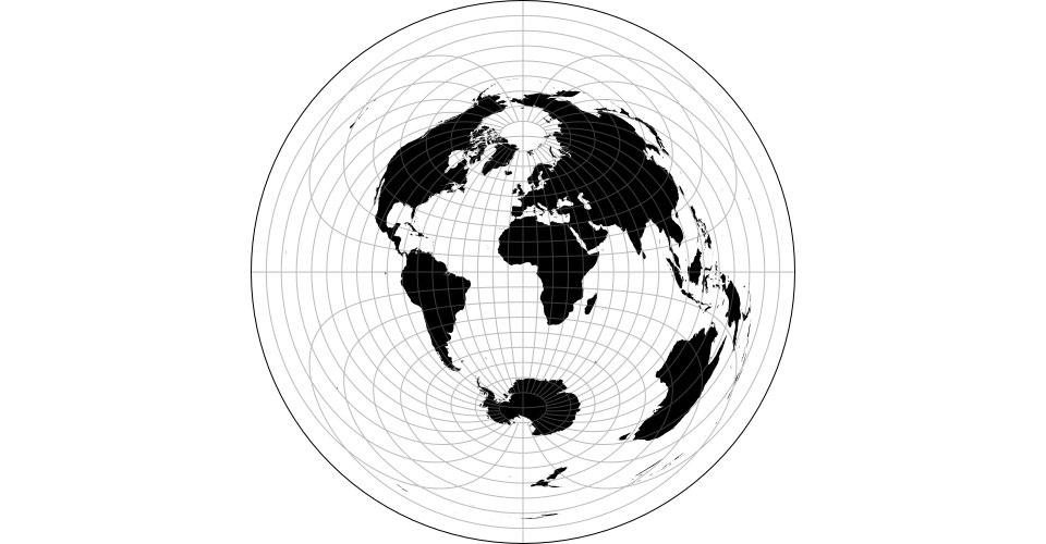 The azimuthal equidistant projection.
# d3.geoGnomonic() <>
The azimuthal equidistant projection.
# d3.geoGnomonic() <>
# d3.geoGnomonicRaw
 The gnomonic projection.
# d3.geoOrthographic() <>
The gnomonic projection.
# d3.geoOrthographic() <>
# d3.geoOrthographicRaw
 The orthographic projection.
# d3.geoStereographic() <>
The orthographic projection.
# d3.geoStereographic() <>
# d3.geoStereographicRaw
 The stereographic projection.
Equal-Earth
# d3.geoEqualEarth() <>
# d3.geoEqualEarthRaw
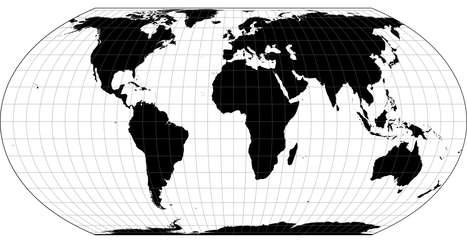 The Equal Earth projection, by Bojan Šavric et al., 2018.
Composite Projections
Composite consist of several projections that are composed into a single display.
The constituent projections have fixed clip, center and rotation, and thus composite projections do not support projection.center, projection.rotate, projection.clipAngle, or projection.clipExtent.
# d3.geoAlbersUsa() <>
 This is a U.S.-centric composite projection of three d3.geoConicEqualArea projections: d3.geoAlbers is used for the lower forty-eight states, and separate conic equal-area projections are used for Alaska and Hawaii.
Note that the scale for Alaska is diminished: it is projected at 0.35× its true relative area.
This diagram by Philippe Rivière illustrates how this projection uses two rectangular insets for Alaska and Hawaii:
This is a U.S.-centric composite projection of three d3.geoConicEqualArea projections: d3.geoAlbers is used for the lower forty-eight states, and separate conic equal-area projections are used for Alaska and Hawaii.
Note that the scale for Alaska is diminished: it is projected at 0.35× its true relative area.
This diagram by Philippe Rivière illustrates how this projection uses two rectangular insets for Alaska and Hawaii:
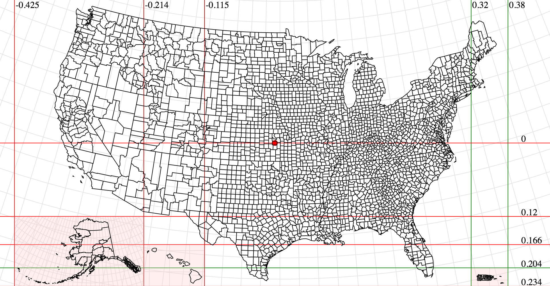 See Albers USA with Territories for an extension to all US territories, and d3-composite-projections for more examples.
Conic Projections
Conic projections project the sphere onto a cone, and then unroll the cone onto the plane.
Conic projections have two standard parallels.
# conic.parallels([parallels]) <>
The two standard parallels that define the map layout in conic projections.
# d3.geoAlbers() <>
 The Albers’ equal area-conic projection.
This is a U.S.-centric configuration of d3.geoConicEqualArea.
# d3.geoConicConformal() <>
The Albers’ equal area-conic projection.
This is a U.S.-centric configuration of d3.geoConicEqualArea.
# d3.geoConicConformal() <>
# d3.geoConicConformalRaw(phi0, phi1) <>
 The conic conformal projection.
The parallels default to [30°, 30°] resulting in flat top.
See also conic.parallels.
# d3.geoConicEqualArea() <>
The conic conformal projection.
The parallels default to [30°, 30°] resulting in flat top.
See also conic.parallels.
# d3.geoConicEqualArea() <>
# d3.geoConicEqualAreaRaw(phi0, phi1) <>
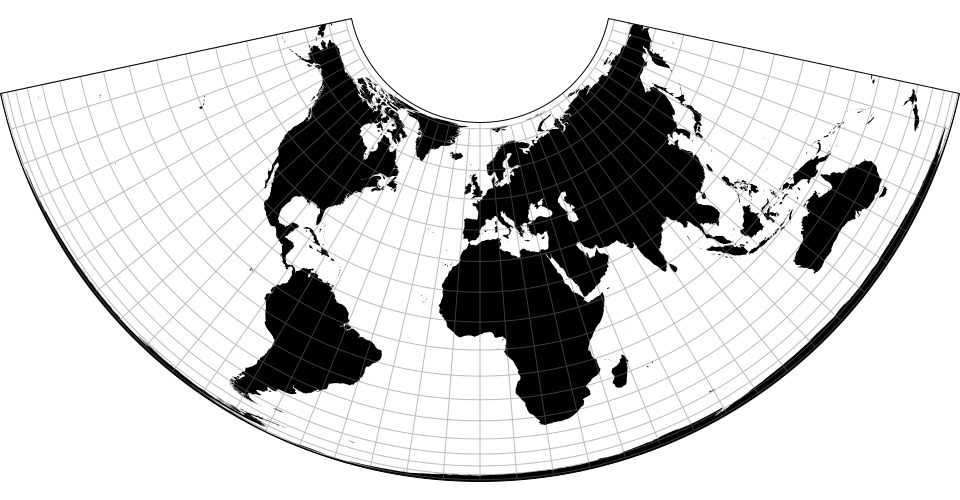 The Albers’ equal-area conic projection.
See also conic.parallels.
# d3.geoConicEquidistant() <>
The Albers’ equal-area conic projection.
See also conic.parallels.
# d3.geoConicEquidistant() <>
# d3.geoConicEquidistantRaw(phi0, phi1) <>
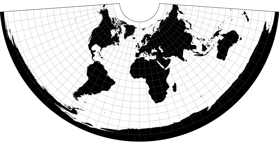 The conic equidistant projection.
See also conic.parallels.
The conic equidistant projection.
See also conic.parallels.
Cylindrical Projections
Cylindrical projections project the sphere onto a containing cylinder, and then unroll the cylinder onto the plane.
Pseudocylindrical projections are a generalization of cylindrical projections.
# d3.geoEquirectangular() <>
# d3.geoEquirectangularRaw
 The equirectangular (plate carrée) projection.
# d3.geoMercator() <>
The equirectangular (plate carrée) projection.
# d3.geoMercator() <>
# d3.geoMercatorRaw
 The spherical Mercator projection.
Defines a default projection.clipExtent such that the world is projected to a square, clipped to approximately ±85° latitude.
# d3.geoTransverseMercator() <>
The spherical Mercator projection.
Defines a default projection.clipExtent such that the world is projected to a square, clipped to approximately ±85° latitude.
# d3.geoTransverseMercator() <>
# d3.geoTransverseMercatorRaw
 The transverse spherical Mercator projection.
Defines a default projection.clipExtent such that the world is projected to a square, clipped to approximately ±85° latitude.
# d3.geoNaturalEarth1() <>
The transverse spherical Mercator projection.
Defines a default projection.clipExtent such that the world is projected to a square, clipped to approximately ±85° latitude.
# d3.geoNaturalEarth1() <>
# d3.geoNaturalEarth1Raw
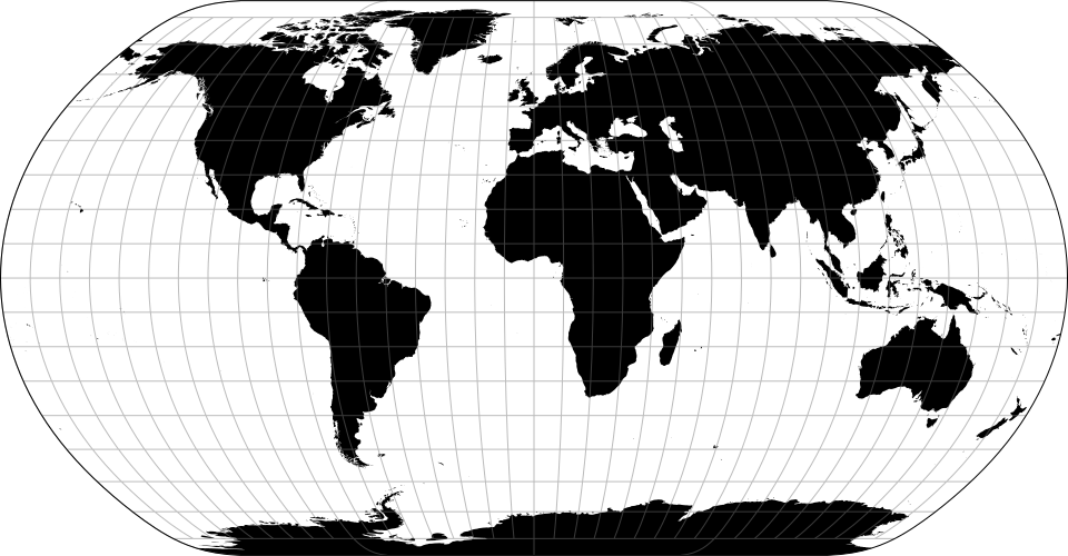 The Natural Earth projection is a pseudocylindrical projection designed by Tom Patterson.
It is neither conformal nor equal-area, but appealing to the eye for small-scale maps of the whole world.
The Natural Earth projection is a pseudocylindrical projection designed by Tom Patterson.
It is neither conformal nor equal-area, but appealing to the eye for small-scale maps of the whole world.
Raw Projections
Raw projections are point transformation functions that are used to implement custom projections; they typically passed to d3.geoProjection or d3.geoProjectionMutator.
They are exposed here to facilitate the derivation of related projections.
Raw projections take spherical coordinates [lambda, phi] in radians (not degrees!) and return a point [x, y], typically in the unit square centered around the origin.
# project(lambda, phi)
Projects the specified point [lambda, phi] in radians, returning a new point [x, y] in unitless coordinates.
# project.invert(x, y)
The inverse of project.
# d3.geoProjection(project) <>
Constructs a new projection from the specified raw projection, project.
The project function takes the longitude and latitude of a given point in radians, often referred to as lambda and phi (f), and returns a two-element array [x, y] representing its unit projection.
The project function does not need to scale or translate the point, as these are applied automatically by projection.scale, projection.translate, and projection.center.
Likewise, the project function does not need to perform any spherical rotation, as projection.rotate is applied prior to projection.
For example, a spherical Mercator projection can be implemented as:
var mercator = d3.geoProjection(function(x, y) {
return [x, Math.log(Math.tan(Math.PI / 4 + y / 2))];
});
If the project function exposes an invert method, the returned projection will also expose projection.invert.
# d3.geoProjectionMutator(factory) <>
Constructs a new projection from the specified raw projection factory and returns a mutate function to call whenever the raw projection changes.
The factory must return a raw projection.
The returned mutate function returns the wrapped projection.
For example, a conic projection typically has two configurable parallels.
A suitable factory function, such as d3.geoConicEqualAreaRaw, would have the form:
// y0 and y1 represent two parallels
function conicFactory(phi0, phi1) {
return function conicRaw(lambda, phi) {
return […, …];
};
}
Using d3.geoProjectionMutator, you can implement a standard projection that allows the parallels to be changed, reassigning the raw projection used internally by d3.geoProjection:
function conicCustom() {
var phi0 = 29.5,
phi1 = 45.5,
mutate = d3.geoProjectionMutator(conicFactory),
projection = mutate(phi0, phi1);
projection.parallels = function(_) {
return arguments.length ? mutate(phi0 = +_[0], phi1 = +_[1]) : [phi0, phi1];
};
return projection;
}
When creating a mutable projection, the mutate function is typically not exposed.
Spherical Math
# d3.geoArea(object) <>
Returns the spherical area of the specified GeoJSON object in steradians.
This is the spherical equivalent of path.area.
# d3.geoBounds(object) <>
Returns the spherical bounding box for the specified GeoJSON object.
The bounding box is represented by a two-dimensional array: [[left, bottom], [right, top]], where left is the minimum longitude, bottom is the minimum latitude, right is maximum longitude, and top is the maximum latitude.
All coordinates are given in degrees.
(Note that in projected planar coordinates, the minimum latitude is typically the maximum y-value, and the maximum latitude is typically the minimum y-value.) This is the spherical equivalent of path.bounds.
# d3.geoCentroid(object) <>
Returns the spherical centroid of the specified GeoJSON object.
This is the spherical equivalent of path.centroid.
# d3.geoDistance(a, b) <>
Returns the great-arc distance in radians between the two points a and b.
Each point must be specified as a two-element array [longitude, latitude] in degrees.
This is the spherical equivalent of path.measure given a LineString of two points.
# d3.geoLength(object) <>
Returns the great-arc length of the specified GeoJSON object in radians.
For polygons, returns the perimeter of the exterior ring plus that of any interior rings.
This is the spherical equivalent of path.measure.
# d3.geoInterpolate(a, b) <>
Returns an interpolator function given two points a and b.
Each point must be specified as a two-element array [longitude, latitude] in degrees.
The returned interpolator function takes a single argument t, where t is a number ranging from 0 to 1; a value of 0 returns the point a, while a value of 1 returns the point b.
Intermediate values interpolate from a to b along the great arc that passes through both a and b.
If a and b are antipodes, an arbitrary great arc is chosen.
# d3.geoContains(object, point) <>
Returns true if and only if the specified GeoJSON object contains the specified point, or false if the object does not contain the point.
The point must be specified as a two-element array [longitude, latitude] in degrees.
For Point and MultiPoint geometries, an exact test is used; for a Sphere, true is always returned; for other geometries, an epsilon threshold is applied.
# d3.geoRotation(angles) <>
Returns a rotation function for the given angles, which must be a two- or three-element array of numbers [lambda, phi, gamma] specifying the rotation angles in degrees about each spherical axis.
(These correspond to yaw, pitch and roll.) If the rotation angle gamma is omitted, it defaults to 0.
See also projection.rotate.
# rotation(point) <>
Returns a new array [longitude, latitude] in degrees representing the rotated point of the given point.
The point must be specified as a two-element array [longitude, latitude] in degrees.
# rotation.invert(point) <>
Returns a new array [longitude, latitude] in degrees representing the point of the given rotated point; the inverse of rotation.
The point must be specified as a two-element array [longitude, latitude] in degrees.
Spherical Shapes
To generate a great arc (a segment of a great circle), simply pass a GeoJSON LineString geometry object to a d3.geoPath.
D3’s projections use great-arc interpolation for intermediate points, so there’s no need for a great arc shape generator.
# d3.geoCircle() <>
Returns a new circle generator.
# circle(arguments…) <>
Returns a new GeoJSON geometry object of type “Polygon” approximating a circle on the surface of a sphere, with the current center, radius and precision.
Any arguments are passed to the accessors.
# circle.center([center]) <>
If center is specified, sets the circle center to the specified point [longitude, latitude] in degrees, and returns this circle generator.
The center may also be specified as a function; this function will be invoked whenever a circle is generated, being passed any arguments passed to the circle generator.
If center is not specified, returns the current center accessor, which defaults to:
function center() {
return [0, 0];
}
# circle.radius([radius]) <>
If radius is specified, sets the circle radius to the specified angle in degrees, and returns this circle generator.
The radius may also be specified as a function; this function will be invoked whenever a circle is generated, being passed any arguments passed to the circle generator.
If radius is not specified, returns the current radius accessor, which defaults to:
function radius() {
return 90;
}
# circle.precision([angle]) <>
If precision is specified, sets the circle precision to the specified angle in degrees, and returns this circle generator.
The precision may also be specified as a function; this function will be invoked whenever a circle is generated, being passed any arguments passed to the circle generator.
If precision is not specified, returns the current precision accessor, which defaults to:
function precision() {
return 6;
}
Small circles do not follow great arcs and thus the generated polygon is only an approximation.
Specifying a smaller precision angle improves the accuracy of the approximate polygon, but also increase the cost to generate and render it.
# d3.geoGraticule() <>
Constructs a geometry generator for creating graticules: a uniform grid of meridians and parallels for showing projection distortion.
The default graticule has meridians and parallels every 10° between ±80° latitude; for the polar regions, there are meridians every 90°.
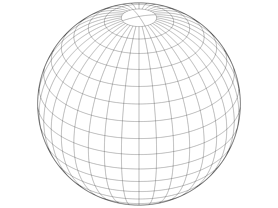 # graticule() <>
Returns a GeoJSON MultiLineString geometry object representing all meridians and parallels for this graticule.
# graticule.lines() <>
Returns an array of GeoJSON LineString geometry objects, one for each meridian or parallel for this graticule.
# graticule.outline() <>
Returns a GeoJSON Polygon geometry object representing the outline of this graticule, i.e.
along the meridians and parallels defining its extent.
# graticule.extent([extent]) <>
If extent is specified, sets the major and minor extents of this graticule.
If extent is not specified, returns the current minor extent, which defaults to -180°, -80° - e, 180°, 80° + e.
# graticule.extentMajor([extent]) <>
If extent is specified, sets the major extent of this graticule.
If extent is not specified, returns the current major extent, which defaults to -180°, -90° + e, 180°, 90° - e.
# graticule.extentMinor([extent]) <>
If extent is specified, sets the minor extent of this graticule.
If extent is not specified, returns the current minor extent, which defaults to -180°, -80° - e, 180°, 80° + e.
# graticule.step([step]) <>
If step is specified, sets the major and minor step for this graticule.
If step is not specified, returns the current minor step, which defaults to 10°, 10°.
# graticule.stepMajor([step]) <>
If step is specified, sets the major step for this graticule.
If step is not specified, returns the current major step, which defaults to 90°, 360°.
# graticule.stepMinor([step]) <>
If step is specified, sets the minor step for this graticule.
If step is not specified, returns the current minor step, which defaults to 10°, 10°.
# graticule.precision([angle]) <>
If precision is specified, sets the precision for this graticule, in degrees.
If precision is not specified, returns the current precision, which defaults to 2.5°.
# d3.geoGraticule10() <>
A convenience method for directly generating the default 10° global graticule as a GeoJSON MultiLineString geometry object.
Equivalent to:
function geoGraticule10() {
return d3.geoGraticule()();
}
# graticule() <>
Returns a GeoJSON MultiLineString geometry object representing all meridians and parallels for this graticule.
# graticule.lines() <>
Returns an array of GeoJSON LineString geometry objects, one for each meridian or parallel for this graticule.
# graticule.outline() <>
Returns a GeoJSON Polygon geometry object representing the outline of this graticule, i.e.
along the meridians and parallels defining its extent.
# graticule.extent([extent]) <>
If extent is specified, sets the major and minor extents of this graticule.
If extent is not specified, returns the current minor extent, which defaults to -180°, -80° - e, 180°, 80° + e.
# graticule.extentMajor([extent]) <>
If extent is specified, sets the major extent of this graticule.
If extent is not specified, returns the current major extent, which defaults to -180°, -90° + e, 180°, 90° - e.
# graticule.extentMinor([extent]) <>
If extent is specified, sets the minor extent of this graticule.
If extent is not specified, returns the current minor extent, which defaults to -180°, -80° - e, 180°, 80° + e.
# graticule.step([step]) <>
If step is specified, sets the major and minor step for this graticule.
If step is not specified, returns the current minor step, which defaults to 10°, 10°.
# graticule.stepMajor([step]) <>
If step is specified, sets the major step for this graticule.
If step is not specified, returns the current major step, which defaults to 90°, 360°.
# graticule.stepMinor([step]) <>
If step is specified, sets the minor step for this graticule.
If step is not specified, returns the current minor step, which defaults to 10°, 10°.
# graticule.precision([angle]) <>
If precision is specified, sets the precision for this graticule, in degrees.
If precision is not specified, returns the current precision, which defaults to 2.5°.
# d3.geoGraticule10() <>
A convenience method for directly generating the default 10° global graticule as a GeoJSON MultiLineString geometry object.
Equivalent to:
function geoGraticule10() {
return d3.geoGraticule()();
}
Streams
D3 transforms geometry using a sequence of function calls, rather than materializing intermediate representations, to minimize overhead.
Streams must implement several methods to receive input geometry.
Streams are inherently stateful; the meaning of a point depends on whether the point is inside of a line, and likewise a line is distinguished from a ring by a polygon.
Despite the name “stream”, these method calls are currently synchronous.
# d3.geoStream(object, stream) <>
Streams the specified GeoJSON object to the specified projection stream.
While both features and geometry objects are supported as input, the stream interface only describes the geometry, and thus additional feature properties are not visible to streams.
# stream.point(x, y[, z])
Indicates a point with the specified coordinates x and y (and optionally z).
The coordinate system is unspecified and implementation-dependent; for example, projection streams require spherical coordinates in degrees as input.
Outside the context of a polygon or line, a point indicates a point geometry object (Point or MultiPoint).
Within a line or polygon ring, the point indicates a control point.
# stream.lineStart()
Indicates the start of a line or ring.
Within a polygon, indicates the start of a ring.
The first ring of a polygon is the exterior ring, and is typically clockwise.
Any subsequent rings indicate holes in the polygon, and are typically counterclockwise.
# stream.lineEnd()
Indicates the end of a line or ring.
Within a polygon, indicates the end of a ring.
Unlike GeoJSON, the redundant closing coordinate of a ring is not indicated via point, and instead is implied via lineEnd within a polygon.
Thus, the given polygon input:
{
"type": "Polygon",
"coordinates": [
[[0, 0], [0, 1], [1, 1], [1, 0], [0, 0]]
]
}
Will produce the following series of method calls on the stream:
stream.polygonStart();
stream.lineStart();
stream.point(0, 0);
stream.point(0, 1);
stream.point(1, 1);
stream.point(1, 0);
stream.lineEnd();
stream.polygonEnd();
# stream.polygonStart()
Indicates the start of a polygon.
The first line of a polygon indicates the exterior ring, and any subsequent lines indicate interior holes.
# stream.polygonEnd()
Indicates the end of a polygon.
# stream.sphere()
Indicates the sphere (the globe; the unit sphere centered at 0,0,0).
Transforms
Transforms are a generalization of projections.
Transform implement projection.stream and can be passed to path.projection.
However, they only implement a subset of the other projection methods, and represent arbitrary geometric transformations rather than projections from spherical to planar coordinates.
# d3.geoTransform(methods) <>
Defines an arbitrary transform using the methods defined on the specified methods object.
Any undefined methods will use pass-through methods that propagate inputs to the output stream.
For example, to reflect the y-dimension (see also identity.reflectY):
var reflectY = d3.geoTransform({
point: function(x, y) {
this.stream.point(x, -y);
}
});
Or to define an affine matrix transformation:
function matrix(a, b, c, d, tx, ty) {
return d3.geoTransform({
point: function(x, y) {
this.stream.point(a * x + b * y + tx, c * x + d * y + ty);
}
});
}
# d3.geoIdentity() <>
The identity transform can be used to scale, translate and clip planar geometry.
It implements projection.scale, projection.translate, projection.fitExtent, projection.fitSize, projection.fitWidth, projection.fitHeight, projection.clipExtent, projection.angle, projection.reflectX and projection.reflectY.
Clipping
Projections perform cutting or clipping of geometries in two stages.
# preclip(stream)
Pre-clipping occurs in geographic coordinates.
Cutting along the antimeridian line, or clipping along a small circle are the most common strategies.
See projection.preclip.
# postclip(stream)
Post-clipping occurs on the plane, when a projection is bounded to a certain extent such as a rectangle.
See projection.postclip.
Clipping functions are implemented as transformations of a projection stream.
Pre-clipping operates on spherical coordinates, in radians.
Post-clipping operates on planar coordinates, in pixels.
# d3.geoClipAntimeridian
A clipping function which transforms a stream such that geometries (lines or polygons) that cross the antimeridian line are cut in two, one on each side.
Typically used for pre-clipping.
# d3.geoClipCircle(angle)
Generates a clipping function which transforms a stream such that geometries are bounded by a small circle of radius angle around the projection’s center.
Typically used for pre-clipping.
# d3.geoClipRectangle(x0, y0, x1, y1)
Generates a clipping function which transforms a stream such that geometries are bounded by a rectangle of coordinates [[x0, y0], [x1, y1]].
Typically used for post-clipping.
d3-hierarchy
Many datasets are intrinsically hierarchical.
Consider geographic entities, such as census blocks, census tracts, counties and states; the command structure of businesses and governments; file systems and software packages.
And even non-hierarchical data may be arranged empirically into a hierarchy, as with k-means clustering or phylogenetic trees.
This module implements several popular techniques for visualizing hierarchical data:
Node-link diagrams show topology using discrete marks for nodes and links, such as a circle for each node and a line connecting each parent and child.
The “tidy” tree is delightfully compact, while the dendrogram places leaves at the same level.
(These have both polar and Cartesian forms.) Indented trees are useful for interactive browsing.
Adjacency diagrams show topology through the relative placement of nodes.
They may also encode a quantitative dimension in the area of each node, for example to show revenue or file size.
The “icicle” diagram uses rectangles, while the “sunburst” uses annular segments.
Enclosure diagrams also use an area encoding, but show topology through containment.
A treemap recursively subdivides area into rectangles.
Circle-packing tightly nests circles; this is not as space-efficient as a treemap, but perhaps more readily shows topology.
A good hierarchical visualization facilitates rapid multiscale inference: micro-observations of individual elements and macro-observations of large groups.
Installing
If you use NPM, npm install d3-hierarchy.
Otherwise, download the latest release.
You can also load directly from d3js.org, either as a standalone library or as part of D3.
AMD, CommonJS, and vanilla environments are supported.
In vanilla, a d3 global is exported:
<script src="https://d3js.org/d3-hierarchy.v2.min.js"></script>
<script>
var treemap = d3.treemap();
</script>
API Reference
Hierarchy (Stratify)
Cluster
Tree
Treemap (Treemap Tiling)
Partition
Pack
Hierarchy
Before you can compute a hierarchical layout, you need a root node.
If your data is already in a hierarchical format, such as JSON, you can pass it directly to d3.hierarchy; otherwise, you can rearrange tabular data, such as comma-separated values (CSV), into a hierarchy using d3.stratify.
# d3.hierarchy(data[, children]) · Source, Examples
Constructs a root node from the specified hierarchical data.
The specified data must be an object representing the root node.
For example:
{
"name": "Eve",
"children": [
{
"name": "Cain"
},
{
"name": "Seth",
"children": [
{
"name": "Enos"
},
{
"name": "Noam"
}
]
},
{
"name": "Abel"
},
{
"name": "Awan",
"children": [
{
"name": "Enoch"
}
]
},
{
"name": "Azura"
}
]
}
The specified children accessor function is invoked for each datum, starting with the root data, and must return an iterable of data representing the children, if any.
If the children accessor is not specified, it defaults to:
function children(d) {
return d.children;
}
If data is a Map, it is implicitly converted to the entry [undefined, data], and the children accessor instead defaults to:
function children(d) {
return Array.isArray(d) ? d[1] : null;
}
This allows you to pass the result of d3.group or d3.rollup to d3.hierarchy.
The returned node and each descendant has the following properties:
node.data - the associated data, as specified to the constructor.
node.depth - zero for the root node, and increasing by one for each descendant generation.
node.height - zero for leaf nodes, and the greatest distance from any descendant leaf for internal nodes.
node.parent - the parent node, or null for the root node.
node.children - an array of child nodes, if any; undefined for leaf nodes.
node.value - the summed value of the node and its descendants; optional, see node.sum and node.count.
This method can also be used to test if a node is an instanceof d3.hierarchy and to extend the node prototype.
# node.ancestors() · Source, Examples
Returns the array of ancestors nodes, starting with this node, then followed by each parent up to the root.
# node.descendants() · Source, Examples
Returns the array of descendant nodes, starting with this node, then followed by each child in topological order.
# node.leaves() · Source, Examples
Returns the array of leaf nodes in traversal order; leaves are nodes with no children.
# node.find(filter) · Source
Returns the first node in the hierarchy from this node for which the specified filter returns a truthy value.
undefined if no such node is found.
# node.path(target) · Source, Examples
Returns the shortest path through the hierarchy from this node to the specified target node.
The path starts at this node, ascends to the least common ancestor of this node and the target node, and then descends to the target node.
This is particularly useful for hierarchical edge bundling.
# node.links() · Source, Examples
Returns an array of links for this node and its descendants, where each link is an object that defines source and target properties.
The source of each link is the parent node, and the target is a child node.
# node.sum(value) · Source, Examples
Evaluates the specified value function for this node and each descendant in post-order traversal, and returns this node.
The node.value property of each node is set to the numeric value returned by the specified function plus the combined value of all children.
The function is passed the node’s data, and must return a non-negative number.
The value accessor is evaluated for node and every descendant, including internal nodes; if you only want leaf nodes to have internal value, then return zero for any node with children.
For example, as an alternative to node.count:
root.sum(function(d) { return d.value ? 1 : 0; });
You must call node.sum or node.count before invoking a hierarchical layout that requires node.value, such as d3.treemap.
Since the API supports method chaining, you can invoke node.sum and node.sort before computing the layout, and then subsequently generate an array of all descendant nodes like so:
var treemap = d3.treemap()
.size([width, height])
.padding(2);
var nodes = treemap(root
.sum(function(d) { return d.value; })
.sort(function(a, b) { return b.height - a.height || b.value - a.value; }))
.descendants();
This example assumes that the node data has a value field.
# node.count() · Source, Examples
Computes the number of leaves under this node and assigns it to node.value, and similarly for every descendant of node.
If this node is a leaf, its count is one.
Returns this node.
See also node.sum.
# node.sort(compare) · Source, Examples
Sorts the children of this node, if any, and each of this node’s descendants’ children, in pre-order traversal using the specified compare function, and returns this node.
The specified function is passed two nodes a and b to compare.
If a should be before b, the function must return a value less than zero; if b should be before a, the function must return a value greater than zero; otherwise, the relative order of a and b are not specified.
See array.sort for more.
Unlike node.sum, the compare function is passed two nodes rather than two nodes’ data.
For example, if the data has a value property, this sorts nodes by the descending aggregate value of the node and all its descendants, as is recommended for circle-packing:
root
.sum(function(d) { return d.value; })
.sort(function(a, b) { return b.value - a.value; });
Similarly, to sort nodes by descending height (greatest distance from any descendant leaf) and then descending value, as is recommended for treemaps and icicles:
root
.sum(function(d) { return d.value; })
.sort(function(a, b) { return b.height - a.height || b.value - a.value; });
To sort nodes by descending height and then ascending id, as is recommended for trees and dendrograms:
root
.sum(function(d) { return d.value; })
.sort(function(a, b) { return b.height - a.height || a.id.localeCompare(b.id); });
You must call node.sort before invoking a hierarchical layout if you want the new sort order to affect the layout; see node.sum for an example.
# nodeSymbol.iterator <>
Returns an iterator over the node’s descendants in breadth-first order.
For example:
for (const descendant of node) {
console.log(descendant);
}
# node.each(function[, that]) · Source, Examples
Invokes the specified function for node and each descendant in breadth-first order, such that a given node is only visited if all nodes of lesser depth have already been visited, as well as all preceding nodes of the same depth.
The specified function is passed the current descendant, the zero-based traversal index, and this node.
If that is specified, it is the this context of the callback.
# node.eachAfter(function[, that]) · Source, Examples
Invokes the specified function for node and each descendant in post-order traversal, such that a given node is only visited after all of its descendants have already been visited.
The specified function is passed the current descendant, the zero-based traversal index, and this node.
If that is specified, it is the this context of the callback.
# node.eachBefore(function[, that]) · Source, Examples
Invokes the specified function for node and each descendant in pre-order traversal, such that a given node is only visited after all of its ancestors have already been visited.
The specified function is passed the current descendant, the zero-based traversal index, and this node.
If that is specified, it is the this context of the callback.
# node.copy() · Source, Examples
Return a deep copy of the subtree starting at this node.
(The returned deep copy shares the same data, however.) The returned node is the root of a new tree; the returned node’s parent is always null and its depth is always zero.
Stratify
Consider the following table of relationships:
| Name |
Parent |
| Eve |
|
| Cain |
Eve |
| Seth |
Eve |
| Enos |
Seth |
| Noam |
Seth |
| Abel |
Eve |
| Awan |
Eve |
| Enoch |
Awan |
| Azura |
Eve |
These names are conveniently unique, so we can unambiguously represent the hierarchy as a CSV file:
name,parent
Eve,
Cain,Eve
Seth,Eve
Enos,Seth
Noam,Seth
Abel,Eve
Awan,Eve
Enoch,Awan
Azura,Eve
To parse the CSV using d3.csvParse:
var table = d3.csvParse(text);
This returns:
[
{"name": "Eve", "parent": ""},
{"name": "Cain", "parent": "Eve"},
{"name": "Seth", "parent": "Eve"},
{"name": "Enos", "parent": "Seth"},
{"name": "Noam", "parent": "Seth"},
{"name": "Abel", "parent": "Eve"},
{"name": "Awan", "parent": "Eve"},
{"name": "Enoch", "parent": "Awan"},
{"name": "Azura", "parent": "Eve"}
]
To convert to a hierarchy:
var root = d3.stratify()
.id(function(d) { return d.name; })
.parentId(function(d) { return d.parent; })
(table);
This returns:
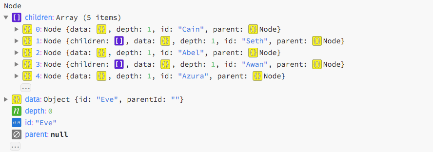 This hierarchy can now be passed to a hierarchical layout, such as d3.tree, for visualization.
# d3.stratify() · Source, Examples
Constructs a new stratify operator with the default settings.
# stratify(data) · Source, Examples
Generates a new hierarchy from the specified tabular data.
# stratify.id([id]) · Source, Examples
If id is specified, sets the id accessor to the given function and returns this stratify operator.
Otherwise, returns the current id accessor, which defaults to:
function id(d) {
return d.id;
}
The id accessor is invoked for each element in the input data passed to the stratify operator, being passed the current datum (d) and the current index (i).
The returned string is then used to identify the node’s relationships in conjunction with the parent id.
For leaf nodes, the id may be undefined; otherwise, the id must be unique.
(Null and the empty string are equivalent to undefined.)
# stratify.parentId([parentId]) · Source, Examples
If parentId is specified, sets the parent id accessor to the given function and returns this stratify operator.
Otherwise, returns the current parent id accessor, which defaults to:
function parentId(d) {
return d.parentId;
}
The parent id accessor is invoked for each element in the input data passed to the stratify operator, being passed the current datum (d) and the current index (i).
The returned string is then used to identify the node’s relationships in conjunction with the id.
For the root node, the parent id should be undefined.
(Null and the empty string are equivalent to undefined.) There must be exactly one root node in the input data, and no circular relationships.
This hierarchy can now be passed to a hierarchical layout, such as d3.tree, for visualization.
# d3.stratify() · Source, Examples
Constructs a new stratify operator with the default settings.
# stratify(data) · Source, Examples
Generates a new hierarchy from the specified tabular data.
# stratify.id([id]) · Source, Examples
If id is specified, sets the id accessor to the given function and returns this stratify operator.
Otherwise, returns the current id accessor, which defaults to:
function id(d) {
return d.id;
}
The id accessor is invoked for each element in the input data passed to the stratify operator, being passed the current datum (d) and the current index (i).
The returned string is then used to identify the node’s relationships in conjunction with the parent id.
For leaf nodes, the id may be undefined; otherwise, the id must be unique.
(Null and the empty string are equivalent to undefined.)
# stratify.parentId([parentId]) · Source, Examples
If parentId is specified, sets the parent id accessor to the given function and returns this stratify operator.
Otherwise, returns the current parent id accessor, which defaults to:
function parentId(d) {
return d.parentId;
}
The parent id accessor is invoked for each element in the input data passed to the stratify operator, being passed the current datum (d) and the current index (i).
The returned string is then used to identify the node’s relationships in conjunction with the id.
For the root node, the parent id should be undefined.
(Null and the empty string are equivalent to undefined.) There must be exactly one root node in the input data, and no circular relationships.
Cluster
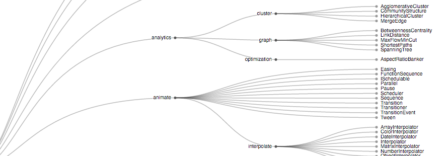 The cluster layout produces dendrograms: node-link diagrams that place leaf nodes of the tree at the same depth.
Dendrograms are typically less compact than tidy trees, but are useful when all the leaves should be at the same level, such as for hierarchical clustering or phylogenetic tree diagrams.
# d3.cluster() · Source, Examples
Creates a new cluster layout with default settings.
# cluster(root)
Lays out the specified root hierarchy, assigning the following properties on root and its descendants:
node.x - the x-coordinate of the node
node.y - the y-coordinate of the node
The coordinates x and y represent an arbitrary coordinate system; for example, you can treat x as an angle and y as a radius to produce a radial layout.
You may want to call root.sort before passing the hierarchy to the cluster layout.
# cluster.size([size])
If size is specified, sets this cluster layout’s size to the specified two-element array of numbers [width, height] and returns this cluster layout.
If size is not specified, returns the current layout size, which defaults to [1, 1].
A layout size of null indicates that a node size will be used instead.
The coordinates x and y represent an arbitrary coordinate system; for example, to produce a radial layout, a size of [360, radius] corresponds to a breadth of 360° and a depth of radius.
# cluster.nodeSize([size])
If size is specified, sets this cluster layout’s node size to the specified two-element array of numbers [width, height] and returns this cluster layout.
If size is not specified, returns the current node size, which defaults to null.
A node size of null indicates that a layout size will be used instead.
When a node size is specified, the root node is always positioned at 0, 0.
# cluster.separation([separation])
If separation is specified, sets the separation accessor to the specified function and returns this cluster layout.
If separation is not specified, returns the current separation accessor, which defaults to:
function separation(a, b) {
return a.parent == b.parent ? 1 : 2;
}
The separation accessor is used to separate neighboring leaves.
The separation function is passed two leaves a and b, and must return the desired separation.
The nodes are typically siblings, though the nodes may be more distantly related if the layout decides to place such nodes adjacent.
The cluster layout produces dendrograms: node-link diagrams that place leaf nodes of the tree at the same depth.
Dendrograms are typically less compact than tidy trees, but are useful when all the leaves should be at the same level, such as for hierarchical clustering or phylogenetic tree diagrams.
# d3.cluster() · Source, Examples
Creates a new cluster layout with default settings.
# cluster(root)
Lays out the specified root hierarchy, assigning the following properties on root and its descendants:
node.x - the x-coordinate of the node
node.y - the y-coordinate of the node
The coordinates x and y represent an arbitrary coordinate system; for example, you can treat x as an angle and y as a radius to produce a radial layout.
You may want to call root.sort before passing the hierarchy to the cluster layout.
# cluster.size([size])
If size is specified, sets this cluster layout’s size to the specified two-element array of numbers [width, height] and returns this cluster layout.
If size is not specified, returns the current layout size, which defaults to [1, 1].
A layout size of null indicates that a node size will be used instead.
The coordinates x and y represent an arbitrary coordinate system; for example, to produce a radial layout, a size of [360, radius] corresponds to a breadth of 360° and a depth of radius.
# cluster.nodeSize([size])
If size is specified, sets this cluster layout’s node size to the specified two-element array of numbers [width, height] and returns this cluster layout.
If size is not specified, returns the current node size, which defaults to null.
A node size of null indicates that a layout size will be used instead.
When a node size is specified, the root node is always positioned at 0, 0.
# cluster.separation([separation])
If separation is specified, sets the separation accessor to the specified function and returns this cluster layout.
If separation is not specified, returns the current separation accessor, which defaults to:
function separation(a, b) {
return a.parent == b.parent ? 1 : 2;
}
The separation accessor is used to separate neighboring leaves.
The separation function is passed two leaves a and b, and must return the desired separation.
The nodes are typically siblings, though the nodes may be more distantly related if the layout decides to place such nodes adjacent.
Tree
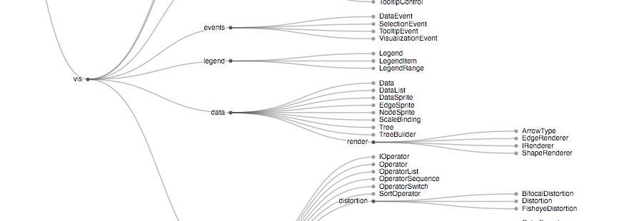 The tree layout produces tidy node-link diagrams of trees using the Reingold–Tilford “tidy” algorithm, improved to run in linear time by Buchheim et al. Tidy trees are typically more compact than dendrograms.
# d3.tree() · Source, Examples
Creates a new tree layout with default settings.
# tree(root)
Lays out the specified root hierarchy, assigning the following properties on root and its descendants:
node.x - the x-coordinate of the node
node.y - the y-coordinate of the node
The coordinates x and y represent an arbitrary coordinate system; for example, you can treat x as an angle and y as a radius to produce a radial layout.
You may want to call root.sort before passing the hierarchy to the tree layout.
# tree.size([size])
If size is specified, sets this tree layout’s size to the specified two-element array of numbers [width, height] and returns this tree layout.
If size is not specified, returns the current layout size, which defaults to [1, 1].
A layout size of null indicates that a node size will be used instead.
The coordinates x and y represent an arbitrary coordinate system; for example, to produce a radial layout, a size of [360, radius] corresponds to a breadth of 360° and a depth of radius.
# tree.nodeSize([size])
If size is specified, sets this tree layout’s node size to the specified two-element array of numbers [width, height] and returns this tree layout.
If size is not specified, returns the current node size, which defaults to null.
A node size of null indicates that a layout size will be used instead.
When a node size is specified, the root node is always positioned at 0, 0.
# tree.separation([separation])
If separation is specified, sets the separation accessor to the specified function and returns this tree layout.
If separation is not specified, returns the current separation accessor, which defaults to:
function separation(a, b) {
return a.parent == b.parent ? 1 : 2;
}
A variation that is more appropriate for radial layouts reduces the separation gap proportionally to the radius:
function separation(a, b) {
return (a.parent == b.parent ? 1 : 2) / a.depth;
}
The separation accessor is used to separate neighboring nodes.
The separation function is passed two nodes a and b, and must return the desired separation.
The nodes are typically siblings, though the nodes may be more distantly related if the layout decides to place such nodes adjacent.
The tree layout produces tidy node-link diagrams of trees using the Reingold–Tilford “tidy” algorithm, improved to run in linear time by Buchheim et al. Tidy trees are typically more compact than dendrograms.
# d3.tree() · Source, Examples
Creates a new tree layout with default settings.
# tree(root)
Lays out the specified root hierarchy, assigning the following properties on root and its descendants:
node.x - the x-coordinate of the node
node.y - the y-coordinate of the node
The coordinates x and y represent an arbitrary coordinate system; for example, you can treat x as an angle and y as a radius to produce a radial layout.
You may want to call root.sort before passing the hierarchy to the tree layout.
# tree.size([size])
If size is specified, sets this tree layout’s size to the specified two-element array of numbers [width, height] and returns this tree layout.
If size is not specified, returns the current layout size, which defaults to [1, 1].
A layout size of null indicates that a node size will be used instead.
The coordinates x and y represent an arbitrary coordinate system; for example, to produce a radial layout, a size of [360, radius] corresponds to a breadth of 360° and a depth of radius.
# tree.nodeSize([size])
If size is specified, sets this tree layout’s node size to the specified two-element array of numbers [width, height] and returns this tree layout.
If size is not specified, returns the current node size, which defaults to null.
A node size of null indicates that a layout size will be used instead.
When a node size is specified, the root node is always positioned at 0, 0.
# tree.separation([separation])
If separation is specified, sets the separation accessor to the specified function and returns this tree layout.
If separation is not specified, returns the current separation accessor, which defaults to:
function separation(a, b) {
return a.parent == b.parent ? 1 : 2;
}
A variation that is more appropriate for radial layouts reduces the separation gap proportionally to the radius:
function separation(a, b) {
return (a.parent == b.parent ? 1 : 2) / a.depth;
}
The separation accessor is used to separate neighboring nodes.
The separation function is passed two nodes a and b, and must return the desired separation.
The nodes are typically siblings, though the nodes may be more distantly related if the layout decides to place such nodes adjacent.
Treemap
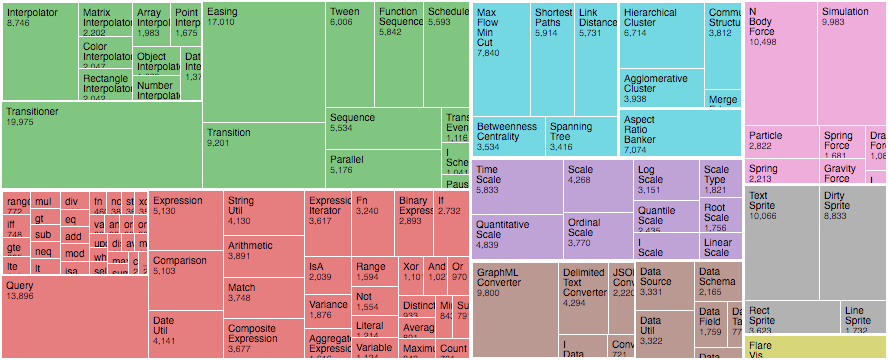 Introduced by Ben Shneiderman in 1991, a treemap recursively subdivides area into rectangles according to each node’s associated value.
D3’s treemap implementation supports an extensible tiling method: the default squarified method seeks to generate rectangles with a golden aspect ratio; this offers better readability and size estimation than slice-and-dice, which simply alternates between horizontal and vertical subdivision by depth.
# d3.treemap() · Source, Examples
Creates a new treemap layout with default settings.
# treemap(root)
Lays out the specified root hierarchy, assigning the following properties on root and its descendants:
node.x0 - the left edge of the rectangle
node.y0 - the top edge of the rectangle
node.x1 - the right edge of the rectangle
node.y1 - the bottom edge of the rectangle
You must call root.sum before passing the hierarchy to the treemap layout.
You probably also want to call root.sort to order the hierarchy before computing the layout.
# treemap.tile([tile])
If tile is specified, sets the tiling method to the specified function and returns this treemap layout.
If tile is not specified, returns the current tiling method, which defaults to d3.treemapSquarify with the golden ratio.
# treemap.size([size])
If size is specified, sets this treemap layout’s size to the specified two-element array of numbers [width, height] and returns this treemap layout.
If size is not specified, returns the current size, which defaults to [1, 1].
# treemap.round([round])
If round is specified, enables or disables rounding according to the given boolean and returns this treemap layout.
If round is not specified, returns the current rounding state, which defaults to false.
# treemap.padding([padding])
If padding is specified, sets the inner and outer padding to the specified number or function and returns this treemap layout.
If padding is not specified, returns the current inner padding function.
# treemap.paddingInner([padding])
If padding is specified, sets the inner padding to the specified number or function and returns this treemap layout.
If padding is not specified, returns the current inner padding function, which defaults to the constant zero.
If padding is a function, it is invoked for each node with children, being passed the current node.
The inner padding is used to separate a node’s adjacent children.
# treemap.paddingOuter([padding])
If padding is specified, sets the top, right, bottom and left padding to the specified number or function and returns this treemap layout.
If padding is not specified, returns the current top padding function.
# treemap.paddingTop([padding])
If padding is specified, sets the top padding to the specified number or function and returns this treemap layout.
If padding is not specified, returns the current top padding function, which defaults to the constant zero.
If padding is a function, it is invoked for each node with children, being passed the current node.
The top padding is used to separate the top edge of a node from its children.
# treemap.paddingRight([padding])
If padding is specified, sets the right padding to the specified number or function and returns this treemap layout.
If padding is not specified, returns the current right padding function, which defaults to the constant zero.
If padding is a function, it is invoked for each node with children, being passed the current node.
The right padding is used to separate the right edge of a node from its children.
# treemap.paddingBottom([padding])
If padding is specified, sets the bottom padding to the specified number or function and returns this treemap layout.
If padding is not specified, returns the current bottom padding function, which defaults to the constant zero.
If padding is a function, it is invoked for each node with children, being passed the current node.
The bottom padding is used to separate the bottom edge of a node from its children.
# treemap.paddingLeft([padding])
If padding is specified, sets the left padding to the specified number or function and returns this treemap layout.
If padding is not specified, returns the current left padding function, which defaults to the constant zero.
If padding is a function, it is invoked for each node with children, being passed the current node.
The left padding is used to separate the left edge of a node from its children.
Introduced by Ben Shneiderman in 1991, a treemap recursively subdivides area into rectangles according to each node’s associated value.
D3’s treemap implementation supports an extensible tiling method: the default squarified method seeks to generate rectangles with a golden aspect ratio; this offers better readability and size estimation than slice-and-dice, which simply alternates between horizontal and vertical subdivision by depth.
# d3.treemap() · Source, Examples
Creates a new treemap layout with default settings.
# treemap(root)
Lays out the specified root hierarchy, assigning the following properties on root and its descendants:
node.x0 - the left edge of the rectangle
node.y0 - the top edge of the rectangle
node.x1 - the right edge of the rectangle
node.y1 - the bottom edge of the rectangle
You must call root.sum before passing the hierarchy to the treemap layout.
You probably also want to call root.sort to order the hierarchy before computing the layout.
# treemap.tile([tile])
If tile is specified, sets the tiling method to the specified function and returns this treemap layout.
If tile is not specified, returns the current tiling method, which defaults to d3.treemapSquarify with the golden ratio.
# treemap.size([size])
If size is specified, sets this treemap layout’s size to the specified two-element array of numbers [width, height] and returns this treemap layout.
If size is not specified, returns the current size, which defaults to [1, 1].
# treemap.round([round])
If round is specified, enables or disables rounding according to the given boolean and returns this treemap layout.
If round is not specified, returns the current rounding state, which defaults to false.
# treemap.padding([padding])
If padding is specified, sets the inner and outer padding to the specified number or function and returns this treemap layout.
If padding is not specified, returns the current inner padding function.
# treemap.paddingInner([padding])
If padding is specified, sets the inner padding to the specified number or function and returns this treemap layout.
If padding is not specified, returns the current inner padding function, which defaults to the constant zero.
If padding is a function, it is invoked for each node with children, being passed the current node.
The inner padding is used to separate a node’s adjacent children.
# treemap.paddingOuter([padding])
If padding is specified, sets the top, right, bottom and left padding to the specified number or function and returns this treemap layout.
If padding is not specified, returns the current top padding function.
# treemap.paddingTop([padding])
If padding is specified, sets the top padding to the specified number or function and returns this treemap layout.
If padding is not specified, returns the current top padding function, which defaults to the constant zero.
If padding is a function, it is invoked for each node with children, being passed the current node.
The top padding is used to separate the top edge of a node from its children.
# treemap.paddingRight([padding])
If padding is specified, sets the right padding to the specified number or function and returns this treemap layout.
If padding is not specified, returns the current right padding function, which defaults to the constant zero.
If padding is a function, it is invoked for each node with children, being passed the current node.
The right padding is used to separate the right edge of a node from its children.
# treemap.paddingBottom([padding])
If padding is specified, sets the bottom padding to the specified number or function and returns this treemap layout.
If padding is not specified, returns the current bottom padding function, which defaults to the constant zero.
If padding is a function, it is invoked for each node with children, being passed the current node.
The bottom padding is used to separate the bottom edge of a node from its children.
# treemap.paddingLeft([padding])
If padding is specified, sets the left padding to the specified number or function and returns this treemap layout.
If padding is not specified, returns the current left padding function, which defaults to the constant zero.
If padding is a function, it is invoked for each node with children, being passed the current node.
The left padding is used to separate the left edge of a node from its children.
Treemap Tiling
Several built-in tiling methods are provided for use with treemap.tile.
# d3.treemapBinary(node, x0, y0, x1, y1) · Source, Examples
Recursively partitions the specified nodes into an approximately-balanced binary tree, choosing horizontal partitioning for wide rectangles and vertical partitioning for tall rectangles.
# d3.treemapDice(node, x0, y0, x1, y1) · Source, Examples
Divides the rectangular area specified by x0, y0, x1, y1 horizontally according the value of each of the specified node’s children.
The children are positioned in order, starting with the left edge (x0) of the given rectangle.
If the sum of the children’s values is less than the specified node’s value (i.e., if the specified node has a non-zero internal value), the remaining empty space will be positioned on the right edge (x1) of the given rectangle.
# d3.treemapSlice(node, x0, y0, x1, y1) · Source, Examples
Divides the rectangular area specified by x0, y0, x1, y1 vertically according the value of each of the specified node’s children.
The children are positioned in order, starting with the top edge (y0) of the given rectangle.
If the sum of the children’s values is less than the specified node’s value (i.e., if the specified node has a non-zero internal value), the remaining empty space will be positioned on the bottom edge (y1) of the given rectangle.
# d3.treemapSliceDice(node, x0, y0, x1, y1) · Source, Examples
If the specified node has odd depth, delegates to treemapSlice; otherwise delegates to treemapDice.
# d3.treemapSquarify(node, x0, y0, x1, y1) · Source, Examples
Implements the squarified treemap algorithm by Bruls et al., which seeks to produce rectangles of a given aspect ratio.
# d3.treemapResquarify(node, x0, y0, x1, y1) · Source, Examples
Like d3.treemapSquarify, except preserves the topology (node adjacencies) of the previous layout computed by d3.treemapResquarify, if there is one and it used the same target aspect ratio.
This tiling method is good for animating changes to treemaps because it only changes node sizes and not their relative positions, thus avoiding distracting shuffling and occlusion.
The downside of a stable update, however, is a suboptimal layout for subsequent updates: only the first layout uses the Bruls et al. squarified algorithm.
# squarify.ratio(ratio) · Source, Examples
Specifies the desired aspect ratio of the generated rectangles.
The ratio must be specified as a number greater than or equal to one.
Note that the orientation of the generated rectangles (tall or wide) is not implied by the ratio; for example, a ratio of two will attempt to produce a mixture of rectangles whose width:height ratio is either 2:1 or 1:2.
(However, you can approximately achieve this result by generating a square treemap at different dimensions, and then stretching the treemap to the desired aspect ratio.) Furthermore, the specified ratio is merely a hint to the tiling algorithm; the rectangles are not guaranteed to have the specified aspect ratio.
If not specified, the aspect ratio defaults to the golden ratio, f = (1 + sqrt(5)) / 2, per Kong et al.
Partition
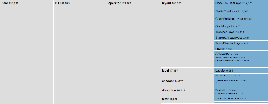 The partition layout produces adjacency diagrams: a space-filling variant of a node-link tree diagram.
Rather than drawing a link between parent and child in the hierarchy, nodes are drawn as solid areas (either arcs or rectangles), and their placement relative to other nodes reveals their position in the hierarchy.
The size of the nodes encodes a quantitative dimension that would be difficult to show in a node-link diagram.
# d3.partition() · Source, Examples
Creates a new partition layout with the default settings.
# partition(root)
Lays out the specified root hierarchy, assigning the following properties on root and its descendants:
node.x0 - the left edge of the rectangle
node.y0 - the top edge of the rectangle
node.x1 - the right edge of the rectangle
node.y1 - the bottom edge of the rectangle
You must call root.sum before passing the hierarchy to the partition layout.
You probably also want to call root.sort to order the hierarchy before computing the layout.
# partition.size([size])
If size is specified, sets this partition layout’s size to the specified two-element array of numbers [width, height] and returns this partition layout.
If size is not specified, returns the current size, which defaults to [1, 1].
# partition.round([round])
If round is specified, enables or disables rounding according to the given boolean and returns this partition layout.
If round is not specified, returns the current rounding state, which defaults to false.
# partition.padding([padding])
If padding is specified, sets the padding to the specified number and returns this partition layout.
If padding is not specified, returns the current padding, which defaults to zero.
The padding is used to separate a node’s adjacent children.
The partition layout produces adjacency diagrams: a space-filling variant of a node-link tree diagram.
Rather than drawing a link between parent and child in the hierarchy, nodes are drawn as solid areas (either arcs or rectangles), and their placement relative to other nodes reveals their position in the hierarchy.
The size of the nodes encodes a quantitative dimension that would be difficult to show in a node-link diagram.
# d3.partition() · Source, Examples
Creates a new partition layout with the default settings.
# partition(root)
Lays out the specified root hierarchy, assigning the following properties on root and its descendants:
node.x0 - the left edge of the rectangle
node.y0 - the top edge of the rectangle
node.x1 - the right edge of the rectangle
node.y1 - the bottom edge of the rectangle
You must call root.sum before passing the hierarchy to the partition layout.
You probably also want to call root.sort to order the hierarchy before computing the layout.
# partition.size([size])
If size is specified, sets this partition layout’s size to the specified two-element array of numbers [width, height] and returns this partition layout.
If size is not specified, returns the current size, which defaults to [1, 1].
# partition.round([round])
If round is specified, enables or disables rounding according to the given boolean and returns this partition layout.
If round is not specified, returns the current rounding state, which defaults to false.
# partition.padding([padding])
If padding is specified, sets the padding to the specified number and returns this partition layout.
If padding is not specified, returns the current padding, which defaults to zero.
The padding is used to separate a node’s adjacent children.
Pack
 Enclosure diagrams use containment (nesting) to represent a hierarchy.
The size of the leaf circles encodes a quantitative dimension of the data.
The enclosing circles show the approximate cumulative size of each subtree, but due to wasted space there is some distortion; only the leaf nodes can be compared accurately.
Although circle packing does not use space as efficiently as a treemap, the “wasted” space more prominently reveals the hierarchical structure.
# d3.pack() · Source, Examples
Creates a new pack layout with the default settings.
# pack(root)
Lays out the specified root hierarchy, assigning the following properties on root and its descendants:
node.x - the x-coordinate of the circle’s center
node.y - the y-coordinate of the circle’s center
node.r - the radius of the circle
You must call root.sum before passing the hierarchy to the pack layout.
You probably also want to call root.sort to order the hierarchy before computing the layout.
# pack.radius([radius])
If radius is specified, sets the pack layout’s radius accessor to the specified function and returns this pack layout.
If radius is not specified, returns the current radius accessor, which defaults to null.
If the radius accessor is null, the radius of each leaf circle is derived from the leaf node.value (computed by node.sum); the radii are then scaled proportionally to fit the layout size.
If the radius accessor is not null, the radius of each leaf circle is specified exactly by the function.
# pack.size([size])
If size is specified, sets this pack layout’s size to the specified two-element array of numbers [width, height] and returns this pack layout.
If size is not specified, returns the current size, which defaults to [1, 1].
# pack.padding([padding])
If padding is specified, sets this pack layout’s padding accessor to the specified number or function and returns this pack layout.
If padding is not specified, returns the current padding accessor, which defaults to the constant zero.
When siblings are packed, tangent siblings will be separated by approximately the specified padding; the enclosing parent circle will also be separated from its children by approximately the specified padding.
If an explicit radius is not specified, the padding is approximate because a two-pass algorithm is needed to fit within the layout size: the circles are first packed without padding; a scaling factor is computed and applied to the specified padding; and lastly the circles are re-packed with padding.
# d3.packSiblings(circles) · Source
Packs the specified array of circles, each of which must have a circle.r property specifying the circle’s radius.
Assigns the following properties to each circle:
circle.x - the x-coordinate of the circle’s center
circle.y - the y-coordinate of the circle’s center
The circles are positioned according to the front-chain packing algorithm by Wang et al.
# d3.packEnclose(circles) · Source, Examples
Computes the smallest circle that encloses the specified array of circles, each of which must have a circle.r property specifying the circle’s radius, and circle.x and circle.y properties specifying the circle’s center.
The enclosing circle is computed using the Matoušek-Sharir-Welzl algorithm.
(See also Apollonius’ Problem.)
Enclosure diagrams use containment (nesting) to represent a hierarchy.
The size of the leaf circles encodes a quantitative dimension of the data.
The enclosing circles show the approximate cumulative size of each subtree, but due to wasted space there is some distortion; only the leaf nodes can be compared accurately.
Although circle packing does not use space as efficiently as a treemap, the “wasted” space more prominently reveals the hierarchical structure.
# d3.pack() · Source, Examples
Creates a new pack layout with the default settings.
# pack(root)
Lays out the specified root hierarchy, assigning the following properties on root and its descendants:
node.x - the x-coordinate of the circle’s center
node.y - the y-coordinate of the circle’s center
node.r - the radius of the circle
You must call root.sum before passing the hierarchy to the pack layout.
You probably also want to call root.sort to order the hierarchy before computing the layout.
# pack.radius([radius])
If radius is specified, sets the pack layout’s radius accessor to the specified function and returns this pack layout.
If radius is not specified, returns the current radius accessor, which defaults to null.
If the radius accessor is null, the radius of each leaf circle is derived from the leaf node.value (computed by node.sum); the radii are then scaled proportionally to fit the layout size.
If the radius accessor is not null, the radius of each leaf circle is specified exactly by the function.
# pack.size([size])
If size is specified, sets this pack layout’s size to the specified two-element array of numbers [width, height] and returns this pack layout.
If size is not specified, returns the current size, which defaults to [1, 1].
# pack.padding([padding])
If padding is specified, sets this pack layout’s padding accessor to the specified number or function and returns this pack layout.
If padding is not specified, returns the current padding accessor, which defaults to the constant zero.
When siblings are packed, tangent siblings will be separated by approximately the specified padding; the enclosing parent circle will also be separated from its children by approximately the specified padding.
If an explicit radius is not specified, the padding is approximate because a two-pass algorithm is needed to fit within the layout size: the circles are first packed without padding; a scaling factor is computed and applied to the specified padding; and lastly the circles are re-packed with padding.
# d3.packSiblings(circles) · Source
Packs the specified array of circles, each of which must have a circle.r property specifying the circle’s radius.
Assigns the following properties to each circle:
circle.x - the x-coordinate of the circle’s center
circle.y - the y-coordinate of the circle’s center
The circles are positioned according to the front-chain packing algorithm by Wang et al.
# d3.packEnclose(circles) · Source, Examples
Computes the smallest circle that encloses the specified array of circles, each of which must have a circle.r property specifying the circle’s radius, and circle.x and circle.y properties specifying the circle’s center.
The enclosing circle is computed using the Matoušek-Sharir-Welzl algorithm.
(See also Apollonius’ Problem.)
d3-interpolate
This module provides a variety of interpolation methods for blending between two values.
Values may be numbers, colors, strings, arrays, or even deeply-nested objects.
For example:
var i = d3.interpolateNumber(10, 20);
i(0.0); // 10
i(0.2); // 12
i(0.5); // 15
i(1.0); // 20
The returned function i is called an interpolator.
Given a starting value a and an ending value b, it takes a parameter t in the domain [0, 1] and returns the corresponding interpolated value between a and b.
An interpolator typically returns a value equivalent to a at t = 0 and a value equivalent to b at t = 1.
You can interpolate more than just numbers.
To find the perceptual midpoint between steelblue and brown:
d3.interpolateLab("steelblue", "brown")(0.5); // "rgb(142, 92, 109)"
Here’s a more elaborate example demonstrating type inference used by interpolate:
var i = d3.interpolate({colors: ["red", "blue"]}, {colors: ["white", "black"]});
i(0.0); // {colors: ["rgb(255, 0, 0)", "rgb(0, 0, 255)"]}
i(0.5); // {colors: ["rgb(255, 128, 128)", "rgb(0, 0, 128)"]}
i(1.0); // {colors: ["rgb(255, 255, 255)", "rgb(0, 0, 0)"]}
Note that the generic value interpolator detects not only nested objects and arrays, but also color strings and numbers embedded in strings!
Installing
If you use NPM, npm install d3-interpolate.
Otherwise, download the latest release.
You can also load directly from d3js.org, either as a standalone library or as part of D3.
AMD, CommonJS, and vanilla environments are supported.
In vanilla, a d3 global is exported.
(If using color interpolation, also load d3-color.)
<script src="https://d3js.org/d3-color.v2.min.js"></script>
<script src="https://d3js.org/d3-interpolate.v2.min.js"></script>
<script>
var interpolate = d3.interpolateRgb("steelblue", "brown");
</script>
API Reference
# d3.interpolate(a, b) · Source, Examples
Returns an interpolator between the two arbitrary values a and b.
The interpolator implementation is based on the type of the end value b, using the following algorithm:
If b is null, undefined or a boolean, use the constant b.
If b is a number, use interpolateNumber.
If b is a color or a string coercible to a color, use interpolateRgb.
If b is a date, use interpolateDate.
If b is a string, use interpolateString.
If b is a typed array of numbers, use interpolateNumberArray.
If b is a generic array, use interpolateArray.
If b is coercible to a number, use interpolateNumber.
Use interpolateObject.
Based on the chosen interpolator, a is coerced to the suitable corresponding type.
# d3.interpolateNumber(a, b) · Source, Examples
Returns an interpolator between the two numbers a and b.
The returned interpolator is equivalent to:
function interpolator(t) {
return a * (1 - t) + b * t;
}
Caution: avoid interpolating to or from the number zero when the interpolator is used to generate a string.
When very small values are stringified, they may be converted to scientific notation, which is an invalid attribute or style property value in older browsers.
For example, the number 0.0000001 is converted to the string "1e-7".
This is particularly noticeable with interpolating opacity.
To avoid scientific notation, start or end the transition at 1e-6: the smallest value that is not stringified in scientific notation.
# d3.interpolateRound(a, b) · Source, Examples
Returns an interpolator between the two numbers a and b; the interpolator is similar to interpolateNumber, except it will round the resulting value to the nearest integer.
# d3.interpolateString(a, b) · Source, Examples
Returns an interpolator between the two strings a and b.
The string interpolator finds numbers embedded in a and b, where each number is of the form understood by JavaScript.
A few examples of numbers that will be detected within a string: -1, 42, 3.14159, and 6.0221413e+23.
For each number embedded in b, the interpolator will attempt to find a corresponding number in a.
If a corresponding number is found, a numeric interpolator is created using interpolateNumber.
The remaining parts of the string b are used as a template: the static parts of the string b remain constant for the interpolation, with the interpolated numeric values embedded in the template.
For example, if a is "300 12px sans-serif", and b is "500 36px Comic-Sans", two embedded numbers are found.
The remaining static parts (of string b) are a space between the two numbers (" "), and the suffix ("px Comic-Sans").
The result of the interpolator at t = 0.5 is "400 24px Comic-Sans".
# d3.interpolateDate(a, b) · Source, Examples
Returns an interpolator between the two dates a and b.
Note: no defensive copy of the returned date is created; the same Date instance is returned for every evaluation of the interpolator.
No copy is made for performance reasons; interpolators are often part of the inner loop of animated transitions.
# d3.interpolateArray(a, b) · Source, Examples
Returns an interpolator between the two arrays a and b.
If b is a typed array (e.g., Float64Array), interpolateNumberArray is called instead.
Internally, an array template is created that is the same length as b.
For each element in b, if there exists a corresponding element in a, a generic interpolator is created for the two elements using interpolate.
If there is no such element, the static value from b is used in the template.
Then, for the given parameter t, the template’s embedded interpolators are evaluated.
The updated array template is then returned.
For example, if a is the array [0, 1] and b is the array [1, 10, 100], then the result of the interpolator for t = 0.5 is the array [0.5, 5.5, 100].
Note: no defensive copy of the template array is created; modifications of the returned array may adversely affect subsequent evaluation of the interpolator.
No copy is made for performance reasons; interpolators are often part of the inner loop of animated transitions.
# d3.interpolateNumberArray(a, b) · Source, Examples
Returns an interpolator between the two arrays of numbers a and b.
Internally, an array template is created that is the same type and length as b.
For each element in b, if there exists a corresponding element in a, the values are directly interpolated in the array template.
If there is no such element, the static value from b is copied.
The updated array template is then returned.
Note: For performance reasons, no defensive copy is made of the template array and the arguments a and b; modifications of these arrays may affect subsequent evaluation of the interpolator.
# d3.interpolateObject(a, b) · Source, Examples
Returns an interpolator between the two objects a and b.
Internally, an object template is created that has the same properties as b.
For each property in b, if there exists a corresponding property in a, a generic interpolator is created for the two elements using interpolate.
If there is no such property, the static value from b is used in the template.
Then, for the given parameter t, the template's embedded interpolators are evaluated and the updated object template is then returned.
For example, if a is the object {x: 0, y: 1} and b is the object {x: 1, y: 10, z: 100}, the result of the interpolator for t = 0.5 is the object {x: 0.5, y: 5.5, z: 100}.
Object interpolation is particularly useful for dataspace interpolation, where data is interpolated rather than attribute values.
For example, you can interpolate an object which describes an arc in a pie chart, and then use d3.arc to compute the new SVG path data.
Note: no defensive copy of the template object is created; modifications of the returned object may adversely affect subsequent evaluation of the interpolator.
No copy is made for performance reasons; interpolators are often part of the inner loop of animated transitions.
# d3.interpolateTransformCss(a, b) · Source, Examples
Returns an interpolator between the two 2D CSS transforms represented by a and b.
Each transform is decomposed to a standard representation of translate, rotate, x-skew and scale; these component transformations are then interpolated.
This behavior is standardized by CSS: see matrix decomposition for animation.
# d3.interpolateTransformSvg(a, b) · Source, Examples
Returns an interpolator between the two 2D SVG transforms represented by a and b.
Each transform is decomposed to a standard representation of translate, rotate, x-skew and scale; these component transformations are then interpolated.
This behavior is standardized by CSS: see matrix decomposition for animation.
# d3.interpolateZoom(a, b) · Source, Examples
Returns an interpolator between the two views a and b of a two-dimensional plane, based on “Smooth and efficient zooming and panning” by Jarke J.
van Wijk and Wim A.A.
Nuij.
Each view is defined as an array of three numbers: cx, cy and width.
The first two coordinates cx, cy represent the center of the viewport; the last coordinate width represents the size of the viewport.
The returned interpolator exposes a duration property which encodes the recommended transition duration in milliseconds.
This duration is based on the path length of the curved trajectory through x,y space.
If you want a slower or faster transition, multiply this by an arbitrary scale factor (V as described in the original paper).
# interpolateZoom.rho(rho) · Source
Given a zoom interpolator, returns a new zoom interpolator using the specified curvature rho.
When rho is close to 0, the interpolator is almost linear.
The default curvature is sqrt(2).
# d3.interpolateDiscrete(values) · Source, Examples
Returns a discrete interpolator for the given array of values.
The returned interpolator maps t in [0, 1 / n) to values[0], t in [1 / n, 2 / n) to values[1], and so on, where n = values.length.
In effect, this is a lightweight quantize scale with a fixed domain of [0, 1].
Sampling
# d3.quantize(interpolator, n) · Source, Examples
Returns n uniformly-spaced samples from the specified interpolator, where n is an integer greater than one.
The first sample is always at t = 0, and the last sample is always at t = 1.
This can be useful in generating a fixed number of samples from a given interpolator, such as to derive the range of a quantize scale from a continuous interpolator.
Caution: this method will not work with interpolators that do not return defensive copies of their output, such as d3.interpolateArray, d3.interpolateDate and d3.interpolateObject.
For those interpolators, you must wrap the interpolator and create a copy for each returned value.
Color Spaces
# d3.interpolateRgb(a, b) · Source, Examples
 Or, with a corrected gamma of 2.2:
 Returns an RGB color space interpolator between the two colors a and b with a configurable gamma.
If the gamma is not specified, it defaults to 1.0.
The colors a and b need not be in RGB; they will be converted to RGB using d3.rgb.
The return value of the interpolator is an RGB string.
# d3.interpolateRgbBasis(colors) · Source, Examples
Returns a uniform nonrational B-spline interpolator through the specified array of colors, which are converted to RGB color space.
Implicit control points are generated such that the interpolator returns colors[0] at t = 0 and colors[colors.length - 1] at t = 1.
Opacity interpolation is not currently supported.
See also d3.interpolateBasis, and see d3-scale-chromatic for examples.
# d3.interpolateRgbBasisClosed(colors) · Source, Examples
Returns a uniform nonrational B-spline interpolator through the specified array of colors, which are converted to RGB color space.
The control points are implicitly repeated such that the resulting spline has cyclical C² continuity when repeated around t in [0,1]; this is useful, for example, to create cyclical color scales.
Opacity interpolation is not currently supported.
See also d3.interpolateBasisClosed, and see d3-scale-chromatic for examples.
# d3.interpolateHsl(a, b) · Source, Examples
Returns an RGB color space interpolator between the two colors a and b with a configurable gamma.
If the gamma is not specified, it defaults to 1.0.
The colors a and b need not be in RGB; they will be converted to RGB using d3.rgb.
The return value of the interpolator is an RGB string.
# d3.interpolateRgbBasis(colors) · Source, Examples
Returns a uniform nonrational B-spline interpolator through the specified array of colors, which are converted to RGB color space.
Implicit control points are generated such that the interpolator returns colors[0] at t = 0 and colors[colors.length - 1] at t = 1.
Opacity interpolation is not currently supported.
See also d3.interpolateBasis, and see d3-scale-chromatic for examples.
# d3.interpolateRgbBasisClosed(colors) · Source, Examples
Returns a uniform nonrational B-spline interpolator through the specified array of colors, which are converted to RGB color space.
The control points are implicitly repeated such that the resulting spline has cyclical C² continuity when repeated around t in [0,1]; this is useful, for example, to create cyclical color scales.
Opacity interpolation is not currently supported.
See also d3.interpolateBasisClosed, and see d3-scale-chromatic for examples.
# d3.interpolateHsl(a, b) · Source, Examples
 Returns an HSL color space interpolator between the two colors a and b.
The colors a and b need not be in HSL; they will be converted to HSL using d3.hsl.
If either color’s hue or saturation is NaN, the opposing color’s channel value is used.
The shortest path between hues is used.
The return value of the interpolator is an RGB string.
# d3.interpolateHslLong(a, b) · Source, Examples
Returns an HSL color space interpolator between the two colors a and b.
The colors a and b need not be in HSL; they will be converted to HSL using d3.hsl.
If either color’s hue or saturation is NaN, the opposing color’s channel value is used.
The shortest path between hues is used.
The return value of the interpolator is an RGB string.
# d3.interpolateHslLong(a, b) · Source, Examples
 Like interpolateHsl, but does not use the shortest path between hues.
# d3.interpolateLab(a, b) · Source, Examples
Like interpolateHsl, but does not use the shortest path between hues.
# d3.interpolateLab(a, b) · Source, Examples
 Returns a CIELAB color space interpolator between the two colors a and b.
The colors a and b need not be in CIELAB; they will be converted to CIELAB using d3.lab.
The return value of the interpolator is an RGB string.
# d3.interpolateHcl(a, b) · Source, Examples
Returns a CIELAB color space interpolator between the two colors a and b.
The colors a and b need not be in CIELAB; they will be converted to CIELAB using d3.lab.
The return value of the interpolator is an RGB string.
# d3.interpolateHcl(a, b) · Source, Examples
 Returns a CIELChab color space interpolator between the two colors a and b.
The colors a and b need not be in CIELChab; they will be converted to CIELChab using d3.hcl.
If either color’s hue or chroma is NaN, the opposing color’s channel value is used.
The shortest path between hues is used.
The return value of the interpolator is an RGB string.
# d3.interpolateHclLong(a, b) · Source, Examples
Returns a CIELChab color space interpolator between the two colors a and b.
The colors a and b need not be in CIELChab; they will be converted to CIELChab using d3.hcl.
If either color’s hue or chroma is NaN, the opposing color’s channel value is used.
The shortest path between hues is used.
The return value of the interpolator is an RGB string.
# d3.interpolateHclLong(a, b) · Source, Examples
 Like interpolateHcl, but does not use the shortest path between hues.
# d3.interpolateCubehelix(a, b) · Source, Examples
Like interpolateHcl, but does not use the shortest path between hues.
# d3.interpolateCubehelix(a, b) · Source, Examples
 Or, with a gamma of 3.0 to emphasize high-intensity values:
 Returns a Cubehelix color space interpolator between the two colors a and b using a configurable gamma.
If the gamma is not specified, it defaults to 1.0.
The colors a and b need not be in Cubehelix; they will be converted to Cubehelix using d3.cubehelix.
If either color’s hue or saturation is NaN, the opposing color’s channel value is used.
The shortest path between hues is used.
The return value of the interpolator is an RGB string.
# d3.interpolateCubehelixLong(a, b) · Source, Examples
Returns a Cubehelix color space interpolator between the two colors a and b using a configurable gamma.
If the gamma is not specified, it defaults to 1.0.
The colors a and b need not be in Cubehelix; they will be converted to Cubehelix using d3.cubehelix.
If either color’s hue or saturation is NaN, the opposing color’s channel value is used.
The shortest path between hues is used.
The return value of the interpolator is an RGB string.
# d3.interpolateCubehelixLong(a, b) · Source, Examples
 Or, with a gamma of 3.0 to emphasize high-intensity values:
 Like interpolateCubehelix, but does not use the shortest path between hues.
# interpolate.gamma(gamma)
Given that interpolate is one of interpolateRgb, interpolateCubehelix or interpolateCubehelixLong, returns a new interpolator factory of the same type using the specified gamma.
For example, to interpolate from purple to orange with a gamma of 2.2 in RGB space:
var interpolator = d3.interpolateRgb.gamma(2.2)("purple", "orange");
See Eric Brasseur’s article, Gamma error in picture scaling, for more on gamma correction.
# d3.interpolateHue(a, b) · Source, Examples
Returns an interpolator between the two hue angles a and b.
If either hue is NaN, the opposing value is used.
The shortest path between hues is used.
The return value of the interpolator is a number in [0, 360).
Like interpolateCubehelix, but does not use the shortest path between hues.
# interpolate.gamma(gamma)
Given that interpolate is one of interpolateRgb, interpolateCubehelix or interpolateCubehelixLong, returns a new interpolator factory of the same type using the specified gamma.
For example, to interpolate from purple to orange with a gamma of 2.2 in RGB space:
var interpolator = d3.interpolateRgb.gamma(2.2)("purple", "orange");
See Eric Brasseur’s article, Gamma error in picture scaling, for more on gamma correction.
# d3.interpolateHue(a, b) · Source, Examples
Returns an interpolator between the two hue angles a and b.
If either hue is NaN, the opposing value is used.
The shortest path between hues is used.
The return value of the interpolator is a number in [0, 360).
Splines
Whereas standard interpolators blend from a starting value a at t = 0 to an ending value b at t = 1, spline interpolators smoothly blend multiple input values for t in [0,1] using piecewise polynomial functions.
Only cubic uniform nonrational B-splines are currently supported, also known as basis splines.
# d3.interpolateBasis(values) · Source, Examples
Returns a uniform nonrational B-spline interpolator through the specified array of values, which must be numbers.
Implicit control points are generated such that the interpolator returns values[0] at t = 0 and values[values.length - 1] at t = 1.
See also d3.curveBasis.
# d3.interpolateBasisClosed(values) · Source, Examples
Returns a uniform nonrational B-spline interpolator through the specified array of values, which must be numbers.
The control points are implicitly repeated such that the resulting one-dimensional spline has cyclical C² continuity when repeated around t in [0,1].
See also d3.curveBasisClosed.
Piecewise
# d3.piecewise([interpolate, ]values) · Source, Examples
Returns a piecewise interpolator, composing interpolators for each adjacent pair of values.
The returned interpolator maps t in [0, 1 / (n - 1)] to interpolate(values[0], values[1]), t in [1 / (n - 1), 2 / (n - 1)] to interpolate(values[1], values[2]), and so on, where n = values.length.
In effect, this is a lightweight linear scale.
For example, to blend through red, green and blue:
var interpolate = d3.piecewise(d3.interpolateRgb.gamma(2.2), ["red", "green", "blue"]);
If interpolate is not specified, defaults to d3.interpolate.
d3-path
Say you have some code that draws to a 2D canvas:
function drawCircle(context, radius) {
context.moveTo(radius, 0);
context.arc(0, 0, radius, 0, 2 * Math.PI);
}
The d3-path module lets you take this exact code and additionally render to SVG.
It works by serializing CanvasPathMethods calls to SVG path data.
For example:
var context = d3.path();
drawCircle(context, 40);
pathElement.setAttribute("d", context.toString());
Now code you write once can be used with both Canvas (for performance) and SVG (for convenience).
For a practical example, see d3-shape.
Installing
If you use NPM, npm install d3-path.
Otherwise, download the latest release.
You can also load directly from d3js.org, either as a standalone library or as part of D3.
AMD, CommonJS, and vanilla environments are supported.
In vanilla, a d3 global is exported:
<script src="https://d3js.org/d3-path.v2.min.js"></script>
<script>
var path = d3.path();
path.moveTo(1, 2);
path.lineTo(3, 4);
path.closePath();
</script>
API Reference
# d3.path() · Source, Examples
Constructs a new path serializer that implements CanvasPathMethods.
# path.moveTo(x, y)
Move to the specified point x, y.
Equivalent to context.moveTo and SVG’s “moveto” command.
# path.closePath()
Ends the current subpath and causes an automatic straight line to be drawn from the current point to the initial point of the current subpath.
Equivalent to context.closePath and SVG’s “closepath” command.
# path.lineTo(x, y)
Draws a straight line from the current point to the specified point x, y.
Equivalent to context.lineTo and SVG’s “lineto” command.
# path.quadraticCurveTo(cpx, cpy, x, y)
Draws a quadratic Bézier segment from the current point to the specified point x, y, with the specified control point cpx, cpy.
Equivalent to context.quadraticCurveTo and SVG’s quadratic Bézier curve commands.
# path.bezierCurveTo(cpx1, cpy1, cpx2, cpy2, x, y)
Draws a cubic Bézier segment from the current point to the specified point x, y, with the specified control points cpx1, cpy1 and cpx2, cpy2.
Equivalent to context.bezierCurveTo and SVG’s cubic Bézier curve commands.
# path.arcTo(x1, y1, x2, y2, radius)
Draws a circular arc segment with the specified radius that starts tangent to the line between the current point and the specified point x1, y1 and ends tangent to the line between the specified points x1, y1 and x2, y2.
If the first tangent point is not equal to the current point, a straight line is drawn between the current point and the first tangent point.
Equivalent to context.arcTo and uses SVG’s elliptical arc curve commands.
# path.arc(x, y, radius, startAngle, endAngle[, anticlockwise])
Draws a circular arc segment with the specified center x, y, radius, startAngle and endAngle.
If anticlockwise is true, the arc is drawn in the anticlockwise direction; otherwise, it is drawn in the clockwise direction.
If the current point is not equal to the starting point of the arc, a straight line is drawn from the current point to the start of the arc.
Equivalent to context.arc and uses SVG’s elliptical arc curve commands.
# path.rect(x, y, w, h)
Creates a new subpath containing just the four points x, y, x + w, y, x + w, y + h, x, y + h, with those four points connected by straight lines, and then marks the subpath as closed.
Equivalent to context.rect and uses SVG’s “lineto” commands.
# path.toString()
Returns the string representation of this path according to SVG’s path data specification.
d3-polygon
This module provides a few basic geometric operations for two-dimensional polygons.
Each polygon is represented as an array of two-element arrays [[x1, y1], [x2, y2], …], and may either be closed (wherein the first and last point are the same) or open (wherein they are not).
Typically polygons are in counterclockwise order, assuming a coordinate system where the origin 0,0 is in the top-left corner.
Installing
If you use NPM, npm install d3-polygon.
Otherwise, download the latest release.
You can also load directly from d3js.org, either as a standalone library or as part of D3.
AMD, CommonJS, and vanilla environments are supported.
In vanilla, a d3 global is exported:
<script src="https://d3js.org/d3-polygon.v2.min.js"></script>
<script>
var hull = d3.polygonHull(points);
</script>
API Reference
# d3.polygonArea(polygon) <>
Returns the signed area of the specified polygon.
If the vertices of the polygon are in counterclockwise order (assuming a coordinate system where the origin 0,0 is in the top-left corner), the returned area is positive; otherwise it is negative, or zero.
# d3.polygonCentroid(polygon) <>
Returns the centroid of the specified polygon.
# d3.polygonHull(points) <>
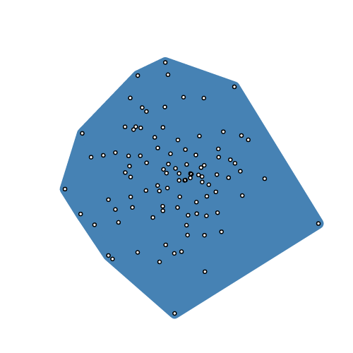 Returns the convex hull of the specified points using Andrew’s monotone chain algorithm.
The returned hull is represented as an array containing a subset of the input points arranged in counterclockwise order.
Returns null if points has fewer than three elements.
# d3.polygonContains(polygon, point) <>
Returns true if and only if the specified point is inside the specified polygon.
# d3.polygonLength(polygon) <>
Returns the length of the perimeter of the specified polygon.
Returns the convex hull of the specified points using Andrew’s monotone chain algorithm.
The returned hull is represented as an array containing a subset of the input points arranged in counterclockwise order.
Returns null if points has fewer than three elements.
# d3.polygonContains(polygon, point) <>
Returns true if and only if the specified point is inside the specified polygon.
# d3.polygonLength(polygon) <>
Returns the length of the perimeter of the specified polygon.
d3-quadtree
A quadtree recursively partitions two-dimensional space into squares, dividing each square into four equally-sized squares.
Each distinct point exists in a unique leaf node; coincident points are represented by a linked list.
Quadtrees can accelerate various spatial operations, such as the Barnes–Hut approximation for computing many-body forces, collision detection, and searching for nearby points.


Installing
If you use NPM, npm install d3-quadtree.
Otherwise, download the latest release.
You can also load directly from d3js.org, either as a standalone library or as part of D3.
AMD, CommonJS, and vanilla environments are supported.
In vanilla, a d3 global is exported:
<script src="https://d3js.org/d3-quadtree.v1.min.js"></script>
<script>
var quadtree = d3.quadtree();
</script>
API Reference
# d3.quadtree([data[, x, y]])
<>
Creates a new, empty quadtree with an empty extent and the default x- and y-accessors.
If data is specified, adds the specified array of data to the quadtree.
This is equivalent to:
var tree = d3.quadtree()
.addAll(data);
If x and y are also specified, sets the x- and y- accessors to the specified functions before adding the specified array of data to the quadtree, equivalent to:
var tree = d3.quadtree()
.x(x)
.y(y)
.addAll(data);
# quadtree.x([x]) <>
If x is specified, sets the current x-coordinate accessor and returns the quadtree.
If x is not specified, returns the current x-accessor, which defaults to:
function x(d) {
return d[0];
}
The x-acccessor is used to derive the x-coordinate of data when adding to and removing from the tree.
It is also used when finding to re-access the coordinates of data previously added to the tree; therefore, the x- and y-accessors must be consistent, returning the same value given the same input.
# quadtree.y([y])
<>
If y is specified, sets the current y-coordinate accessor and returns the quadtree.
If y is not specified, returns the current y-accessor, which defaults to:
function y(d) {
return d[1];
}
The y-acccessor is used to derive the y-coordinate of data when adding to and removing from the tree.
It is also used when finding to re-access the coordinates of data previously added to the tree; therefore, the x- and y-accessors must be consistent, returning the same value given the same input.
# quadtree.extent([extent])
<>
If extent is specified, expands the quadtree to cover the specified points [[x0, y0], [x1, y1]] and returns the quadtree.
If extent is not specified, returns the quadtree’s current extent [[x0, y0], [x1, y1]], where x0 and y0 are the inclusive lower bounds and x1 and y1 are the inclusive upper bounds, or undefined if the quadtree has no extent.
The extent may also be expanded by calling quadtree.cover or quadtree.add.
# quadtree.cover(x, y)
<>
Expands the quadtree to cover the specified point x,y, and returns the quadtree.
If the quadtree’s extent already covers the specified point, this method does nothing.
If the quadtree has an extent, the extent is repeatedly doubled to cover the specified point, wrapping the root node as necessary; if the quadtree is empty, the extent is initialized to the extent [[x, y], [x, y]].
(Rounding is necessary such that if the extent is later doubled, the boundaries of existing quadrants do not change due to floating point error.)
# quadtree.add(datum)
<>
Adds the specified datum to the quadtree, deriving its coordinates x,y using the current x- and y-accessors, and returns the quadtree.
If the new point is outside the current extent of the quadtree, the quadtree is automatically expanded to cover the new point.
# quadtree.addAll(data)
<>
Adds the specified array of data to the quadtree, deriving each element’s coordinates x,y using the current x- and y-accessors, and return this quadtree.
This is approximately equivalent to calling quadtree.add repeatedly:
for (var i = 0, n = data.length; i < n; ++i) {
quadtree.add(data[i]);
}
However, this method results in a more compact quadtree because the extent of the data is computed first before adding the data.
# quadtree.remove(datum)
<>
Removes the specified datum from the quadtree, deriving its coordinates x,y using the current x- and y-accessors, and returns the quadtree.
If the specified datum does not exist in this quadtree, this method does nothing.
# quadtree.removeAll(data)
<>
Removes the specified data from the quadtree, deriving their coordinates x,y using the current x- and y-accessors, and returns the quadtree.
If a specified datum does not exist in this quadtree, it is ignored.
# quadtree.copy()
Returns a copy of the quadtree.
All nodes in the returned quadtree are identical copies of the corresponding node in the quadtree; however, any data in the quadtree is shared by reference and not copied.
# quadtree.root()
<>
Returns the root node of the quadtree.
# quadtree.data()
<>
Returns an array of all data in the quadtree.
# quadtree.size()
<>
Returns the total number of data in the quadtree.
# quadtree.find(x, y[, radius])
<>
Returns the datum closest to the position x,y with the given search radius.
If radius is not specified, it defaults to infinity.
If there is no datum within the search area, returns undefined.
# quadtree.visit(callback)
<>
Visits each node in the quadtree in pre-order traversal, invoking the specified callback with arguments node, x0, y0, x1, y1 for each node, where node is the node being visited, x0, y0 are the lower bounds of the node, and x1, y1 are the upper bounds, and returns the quadtree.
(Assuming that positive x is right and positive y is down, as is typically the case in Canvas and SVG, x0, y0 is the top-left corner and x1, y1 is the lower-right corner; however, the coordinate system is arbitrary, so more formally x0 <= x1 and y0 <= y1.)
If the callback returns true for a given node, then the children of that node are not visited; otherwise, all child nodes are visited.
This can be used to quickly visit only parts of the tree, for example when using the Barnes–Hut approximation.
Note, however, that child quadrants are always visited in sibling order: top-left, top-right, bottom-left, bottom-right.
In cases such as search, visiting siblings in a specific order may be faster.
As an example, the following visits the quadtree and returns all the nodes within a rectangular extent [xmin, ymin, xmax, ymax], ignoring quads that cannot possibly contain any such node:
function search(quadtree, xmin, ymin, xmax, ymax) {
const results = [];
quadtree.visit(function(node, x1, y1, x2, y2) {
if (!node.length) {
do {
var d = node.data;
if (d[0] >= xmin && d[0] < xmax && d[1] >= ymin && d[1] < ymax) {
results.push(d);
}
} while (node = node.next);
}
return x1 >= xmax || y1 >= ymax || x2 < xmin || y2 < ymin;
});
return results;
}
# quadtree.visitAfter(callback)
<>
Visits each node in the quadtree in post-order traversal, invoking the specified callback with arguments node, x0, y0, x1, y1 for each node, where node is the node being visited, x0, y0 are the lower bounds of the node, and x1, y1 are the upper bounds, and returns the quadtree.
(Assuming that positive x is right and positive y is down, as is typically the case in Canvas and SVG, x0, y0 is the top-left corner and x1, y1 is the lower-right corner; however, the coordinate system is arbitrary, so more formally x0 <= x1 and y0 <= y1.) Returns root.
Nodes
Internal nodes of the quadtree are represented as four-element arrays in left-to-right, top-to-bottom order:
0 - the top-left quadrant, if any.
1 - the top-right quadrant, if any.
2 - the bottom-left quadrant, if any.
3 - the bottom-right quadrant, if any.
A child quadrant may be undefined if it is empty.
Leaf nodes are represented as objects with the following properties:
data - the data associated with this point, as passed to quadtree.add.
next - the next datum in this leaf, if any.
The length property may be used to distinguish leaf nodes from internal nodes: it is undefined for leaf nodes, and 4 for internal nodes.
For example, to iterate over all data in a leaf node:
if (!node.length) do console.log(node.data); while (node = node.next);
The point’s x- and y-coordinates must not be modified while the point is in the quadtree.
To update a point’s position, remove the point and then re-add it to the quadtree at the new position.
Alternatively, you may discard the existing quadtree entirely and create a new one from scratch; this may be more efficient if many of the points have moved.
d3-random
Generate random numbers from various distributions.
See the d3-random collection on Observable for examples.
Installing
If you use NPM, npm install d3-random.
Otherwise, download the latest release.
You can also load directly as a standalone library or as part of D3.
ES modules, AMD, CommonJS, and vanilla environments are supported.
In vanilla, a d3 global is exported:
<script src="https://d3js.org/d3-random.v2.min.js"></script>
<script>
var random = d3.randomUniform(1, 10);
</script>
API Reference
# d3.randomUniform([min, ][max]) · Source, Examples
Returns a function for generating random numbers with a uniform distribution.
The minimum allowed value of a returned number is min (inclusive), and the maximum is max (exclusive).
If min is not specified, it defaults to 0; if max is not specified, it defaults to 1.
For example:
d3.randomUniform(6)(); // Returns a number greater than or equal to 0 and less than 6.
d3.randomUniform(1, 5)(); // Returns a number greater than or equal to 1 and less than 5.
# d3.randomInt([min, ][max]) · Source, Examples
Returns a function for generating random integers with a uniform distribution.
The minimum allowed value of a returned number is min (inclusive), and the maximum is max - 1 (inclusive).
If min is not specified, it defaults to 0.
For example:
d3.randomInt(6)(); // Returns an integer greater than or equal to 0 and less than 6.
d3.randomInt(1, 5)(); // Returns an integer greater than or equal to 1 and less than 5.
# d3.randomNormal([mu][, sigma]) · Source, Examples
Returns a function for generating random numbers with a normal (Gaussian) distribution.
The expected value of the generated numbers is mu, with the given standard deviation sigma.
If mu is not specified, it defaults to 0; if sigma is not specified, it defaults to 1.
# d3.randomLogNormal([mu][, sigma]) · Source, Examples
Returns a function for generating random numbers with a log-normal distribution.
The expected value of the random variable’s natural logarithm is mu, with the given standard deviation sigma.
If mu is not specified, it defaults to 0; if sigma is not specified, it defaults to 1.
# d3.randomBates(n) · Source, Examples
Returns a function for generating random numbers with a Bates distribution with n independent variables.
The case of fractional n is handled as with d3.randomIrwinHall, and d3.randomBates(0) is equivalent to d3.randomUniform().
# d3.randomIrwinHall(n) · Source, Examples
Returns a function for generating random numbers with an Irwin–Hall distribution with n independent variables.
If the fractional part of n is non-zero, this is treated as adding d3.randomUniform() times that fractional part to the integral part.
# d3.randomExponential(lambda) · Source, Examples
Returns a function for generating random numbers with an exponential distribution with the rate lambda; equivalent to time between events in a Poisson process with a mean of 1 / lambda.
For example, exponential(1/40) generates random times between events where, on average, one event occurs every 40 units of time.
# d3.randomPareto(alpha) · Source, Examples
Returns a function for generating random numbers with a Pareto distribution with the shape alpha.
The value alpha must be a positive value.
# d3.randomBernoulli(p) · Source, Examples
Returns a function for generating either 1 or 0 according to a Bernoulli distribution with 1 being returned with success probability p and 0 with failure probability q = 1 - p.
The value p is in the range [0, 1].
# d3.randomGeometric(p) · Source, Examples
Returns a function for generating numbers with a geometric distribution with success probability p.
The value p is in the range [0, 1].
# d3.randomBinomial(n, p) · Source, Examples
Returns a function for generating random numbers with a binomial distribution with n the number of trials and p the probability of success in each trial.
The value n is greater or equal to 0, and the value p is in the range [0, 1].
# d3.randomGamma(k, [theta]) · Source, Examples
Returns a function for generating random numbers with a gamma distribution with k the shape parameter and theta the scale parameter.
The value k must be a positive value; if theta is not specified, it defaults to 1.
# d3.randomBeta(alpha, beta) · Source, Examples
Returns a function for generating random numbers with a beta distribution with alpha and beta shape parameters, which must both be positive.
# d3.randomWeibull(k, [a], [b]) · Source, Examples
Returns a function for generating random numbers with one of the generalized extreme value distributions, depending on k:
If k is positive, the Weibull distribution with shape parameter k
If k is zero, the Gumbel distribution
If k is negative, the Fréchet distribution with shape parameter -k
In all three cases, a is the location parameter and b is the scale parameter.
If a is not specified, it defaults to 0; if b is not specified, it defaults to 1.
# d3.randomCauchy([a], [b]) · Source, Examples
Returns a function for generating random numbers with a Cauchy distribution.
a and b have the same meanings and default values as in d3.randomWeibull.
# d3.randomLogistic([a], [b]) · Source, Examples
Returns a function for generating random numbers with a logistic distribution.
a and b have the same meanings and default values as in d3.randomWeibull.
# d3.randomPoisson(lambda) · Source, Examples
Returns a function for generating random numbers with a Poisson distribution with mean lambda.
# random.source(source) · Examples
Returns the same type of function for generating random numbers but where the given random number generator source is used as the source of randomness instead of Math.random.
The given random number generator must implement the same interface as Math.random and only return values in the range [0, 1).
This is useful when a seeded random number generator is preferable to Math.random.
For example:
const d3 = require("d3-random");
const seed = 0.44871573888282423; // any number in [0, 1)
const random = d3.randomNormal.source(d3.randomLcg(seed))(0, 1);
random(); // -0.6253955998897069
# d3.randomLcg([seed]) · Source, Examples
Returns a linear congruential generator; this function can be called repeatedly to obtain pseudorandom values well-distributed on the interval [0,1) and with a long period (up to 1 billion numbers), similar to Math.random.
A seed can be specified as a real number in the interval [0,1) or as any integer.
In the latter case, only the lower 32 bits are considered.
Two generators instanced with the same seed generate the same sequence, allowing to create reproducible pseudo-random experiments.
If the seed is not specified, one is chosen using Math.random.
d3-scale
Scales are a convenient abstraction for a fundamental task in visualization: mapping a dimension of abstract data to a visual representation.
Although most often used for position-encoding quantitative data, such as mapping a measurement in meters to a position in pixels for dots in a scatterplot, scales can represent virtually any visual encoding, such as diverging colors, stroke widths, or symbol size.
Scales can also be used with virtually any type of data, such as named categorical data or discrete data that requires sensible breaks.
For continuous quantitative data, you typically want a linear scale.
(For time series data, a time scale.) If the distribution calls for it, consider transforming data using a power or log scale.
A quantize scale may aid differentiation by rounding continuous data to a fixed set of discrete values; similarly, a quantile scale computes quantiles from a sample population, and a threshold scale allows you to specify arbitrary breaks in continuous data.
For discrete ordinal (ordered) or categorical (unordered) data, an ordinal scale specifies an explicit mapping from a set of data values to a corresponding set of visual attributes (such as colors).
The related band and point scales are useful for position-encoding ordinal data, such as bars in a bar chart or dots in an categorical scatterplot.
This repository does not provide color schemes; see d3-scale-chromatic for color schemes designed to work with d3-scale.
Scales have no intrinsic visual representation.
However, most scales can generate and format ticks for reference marks to aid in the construction of axes.
For a longer introduction, see these recommended tutorials:
Introducing d3-scale by Mike Bostock
Chapter 7.
Scales of Interactive Data Visualization for the Web by Scott Murray
d3: scales, and color. by Jérôme Cukier
Installing
If you use NPM, npm install d3-scale.
Otherwise, download the latest release.
You can also load directly from d3js.org, either as a standalone library or as part of D3.
AMD, CommonJS, and vanilla environments are supported.
In vanilla, a d3 global is exported:
<script src="https://d3js.org/d3-array.v2.min.js"></script>
<script src="https://d3js.org/d3-color.v1.min.js"></script>
<script src="https://d3js.org/d3-format.v1.min.js"></script>
<script src="https://d3js.org/d3-interpolate.v1.min.js"></script>
<script src="https://d3js.org/d3-time.v1.min.js"></script>
<script src="https://d3js.org/d3-time-format.v2.min.js"></script>
<script src="https://d3js.org/d3-scale.v3.min.js"></script>
<script>
var x = d3.scaleLinear();
</script>
(You can omit d3-time and d3-time-format if you’re not using d3.scaleTime or d3.scaleUtc.)
API Reference
Continuous (Linear, Power, Log, Identity, Time, Radial)
Sequential
Diverging
Quantize
Quantile
Threshold
Ordinal (Band, Point)
Continuous Scales
Continuous scales map a continuous, quantitative input domain to a continuous output range.
If the range is also numeric, the mapping may be inverted.
A continuous scale is not constructed directly; instead, try a linear, power, log, identity, radial, time or sequential color scale.
# continuous(value) · Source, Examples
Given a value from the domain, returns the corresponding value from the range.
If the given value is outside the domain, and clamping is not enabled, the mapping may be extrapolated such that the returned value is outside the range.
For example, to apply a position encoding:
var x = d3.scaleLinear()
.domain([10, 130])
.range([0, 960]);
x(20); // 80
x(50); // 320
Or to apply a color encoding:
var color = d3.scaleLinear()
.domain([10, 100])
.range(["brown", "steelblue"]);
color(20); // "#9a3439"
color(50); // "#7b5167"
Or, in shorthand:
var x = d3.scaleLinear([10, 130], [0, 960]);
var color = d3.scaleLinear([10, 100], ["brown", "steelblue"]);
# continuous.invert(value) · Source, Examples
Given a value from the range, returns the corresponding value from the domain.
Inversion is useful for interaction, say to determine the data value corresponding to the position of the mouse.
For example, to invert a position encoding:
var x = d3.scaleLinear()
.domain([10, 130])
.range([0, 960]);
x.invert(80); // 20
x.invert(320); // 50
If the given value is outside the range, and clamping is not enabled, the mapping may be extrapolated such that the returned value is outside the domain.
This method is only supported if the range is numeric.
If the range is not numeric, returns NaN.
For a valid value y in the range, continuous(continuous.invert(y)) approximately equals y; similarly, for a valid value x in the domain, continuous.invert(continuous(x)) approximately equals x.
The scale and its inverse may not be exact due to the limitations of floating point precision.
# continuous.domain([domain]) · Source, Examples
If domain is specified, sets the scale’s domain to the specified array of numbers.
The array must contain two or more elements.
If the elements in the given array are not numbers, they will be coerced to numbers.
If domain is not specified, returns a copy of the scale’s current domain.
Although continuous scales typically have two values each in their domain and range, specifying more than two values produces a piecewise scale.
For example, to create a diverging color scale that interpolates between white and red for negative values, and white and green for positive values, say:
var color = d3.scaleLinear()
.domain([-1, 0, 1])
.range(["red", "white", "green"]);
color(-0.5); // "rgb(255, 128, 128)"
color(+0.5); // "rgb(128, 192, 128)"
Internally, a piecewise scale performs a binary search for the range interpolator corresponding to the given domain value.
Thus, the domain must be in ascending or descending order.
If the domain and range have different lengths N and M, only the first min(N,M) elements in each are observed.
# continuous.range([range]) · Source, Examples
If range is specified, sets the scale’s range to the specified array of values.
The array must contain two or more elements.
Unlike the domain, elements in the given array need not be numbers; any value that is supported by the underlying interpolator will work, though note that numeric ranges are required for invert.
If range is not specified, returns a copy of the scale’s current range.
See continuous.interpolate for more examples.
# continuous.rangeRound([range]) · Source, Examples
Sets the scale’s range to the specified array of values while also setting the scale’s interpolator to interpolateRound.
This is a convenience method equivalent to:
continuous
.range(range)
.interpolate(d3.interpolateRound);
The rounding interpolator is sometimes useful for avoiding antialiasing artifacts, though also consider the shape-rendering “crispEdges” styles.
Note that this interpolator can only be used with numeric ranges.
# continuous.clamp(clamp) · Source, Examples
If clamp is specified, enables or disables clamping accordingly.
If clamping is disabled and the scale is passed a value outside the domain, the scale may return a value outside the range through extrapolation.
If clamping is enabled, the return value of the scale is always within the scale’s range.
Clamping similarly applies to continuous.invert.
For example:
var x = d3.scaleLinear()
.domain([10, 130])
.range([0, 960]);
x(-10); // -160, outside range
x.invert(-160); // -10, outside domain
x.clamp(true);
x(-10); // 0, clamped to range
x.invert(-160); // 10, clamped to domain
If clamp is not specified, returns whether or not the scale currently clamps values to within the range.
# continuous.unknown([value]) · Source, Examples
If value is specified, sets the output value of the scale for undefined (or NaN) input values and returns this scale.
If value is not specified, returns the current unknown value, which defaults to undefined.
# continuous.interpolate(interpolate) · Source, Examples
If interpolate is specified, sets the scale’s range interpolator factory.
This interpolator factory is used to create interpolators for each adjacent pair of values from the range; these interpolators then map a normalized domain parameter t in [0, 1] to the corresponding value in the range.
If factory is not specified, returns the scale’s current interpolator factory, which defaults to d3.interpolate.
See d3-interpolate for more interpolators.
For example, consider a diverging color scale with three colors in the range:
var color = d3.scaleLinear()
.domain([-100, 0, +100])
.range(["red", "white", "green"]);
Two interpolators are created internally by the scale, equivalent to:
var i0 = d3.interpolate("red", "white"),
i1 = d3.interpolate("white", "green");
A common reason to specify a custom interpolator is to change the color space of interpolation.
For example, to use HCL:
var color = d3.scaleLinear()
.domain([10, 100])
.range(["brown", "steelblue"])
.interpolate(d3.interpolateHcl);
Or for Cubehelix with a custom gamma:
var color = d3.scaleLinear()
.domain([10, 100])
.range(["brown", "steelblue"])
.interpolate(d3.interpolateCubehelix.gamma(3));
Note: the default interpolator may reuse return values.
For example, if the range values are objects, then the value interpolator always returns the same object, modifying it in-place.
If the scale is used to set an attribute or style, this is typically acceptable (and desirable for performance); however, if you need to store the scale’s return value, you must specify your own interpolator or make a copy as appropriate.
# continuous.ticks([count])
Returns approximately count representative values from the scale’s domain.
If count is not specified, it defaults to 10.
The returned tick values are uniformly spaced, have human-readable values (such as multiples of powers of 10), and are guaranteed to be within the extent of the domain.
Ticks are often used to display reference lines, or tick marks, in conjunction with the visualized data.
The specified count is only a hint; the scale may return more or fewer values depending on the domain.
See also d3-array’s ticks.
# continuous.tickFormat([count[, specifier]]) · Source, Examples
Returns a number format function suitable for displaying a tick value, automatically computing the appropriate precision based on the fixed interval between tick values.
The specified count should have the same value as the count that is used to generate the tick values.
An optional specifier allows a custom format where the precision of the format is automatically set by the scale as appropriate for the tick interval.
For example, to format percentage change, you might say:
var x = d3.scaleLinear()
.domain([-1, 1])
.range([0, 960]);
var ticks = x.ticks(5),
tickFormat = x.tickFormat(5, "+%");
ticks.map(tickFormat); // ["-100%", "-50%", "+0%", "+50%", "+100%"]
If specifier uses the format type s, the scale will return a SI-prefix format based on the largest value in the domain.
If the specifier already specifies a precision, this method is equivalent to locale.format.
See also d3.tickFormat.
# continuous.nice([count]) · Source, Examples
Extends the domain so that it starts and ends on nice round values.
This method typically modifies the scale’s domain, and may only extend the bounds to the nearest round value.
An optional tick count argument allows greater control over the step size used to extend the bounds, guaranteeing that the returned ticks will exactly cover the domain.
Nicing is useful if the domain is computed from data, say using extent, and may be irregular.
For example, for a domain of [0.201479…, 0.996679…], a nice domain might be [0.2, 1.0].
If the domain has more than two values, nicing the domain only affects the first and last value.
See also d3-array’s tickStep.
Nicing a scale only modifies the current domain; it does not automatically nice domains that are subsequently set using continuous.domain.
You must re-nice the scale after setting the new domain, if desired.
# continuous.copy() · Source, Examples
Returns an exact copy of this scale.
Changes to this scale will not affect the returned scale, and vice versa.
# d3.tickFormat(start, stop, count[, specifier]) · Source, Examples
Returns a number format function suitable for displaying a tick value, automatically computing the appropriate precision based on the fixed interval between tick values, as determined by d3.tickStep.
An optional specifier allows a custom format where the precision of the format is automatically set by the scale as appropriate for the tick interval.
For example, to format percentage change, you might say:
var tickFormat = d3.tickFormat(-1, 1, 5, "+%");
tickFormat(-0.5); // "-50%"
If specifier uses the format type s, the scale will return a SI-prefix format based on the larger absolute value of start and stop.
If the specifier already specifies a precision, this method is equivalent to locale.format.
Linear Scales
# d3.scaleLinear([[domain, ]range]) · Source, Examples
Constructs a new continuous scale with the specified domain and range, the default interpolator and clamping disabled.
If either domain or range are not specified, each defaults to [0, 1].
Linear scales are a good default choice for continuous quantitative data because they preserve proportional differences.
Each range value y can be expressed as a function of the domain value x: y = mx + b.
Power Scales
Power scales are similar to linear scales, except an exponential transform is applied to the input domain value before the output range value is computed.
Each range value y can be expressed as a function of the domain value x: y = mx^k + b, where k is the exponent value.
Power scales also support negative domain values, in which case the input value and the resulting output value are multiplied by -1.
# d3.scalePow([[domain, ]range]) · Source, Examples
Constructs a new continuous scale with the specified domain and range, the exponent 1, the default interpolator and clamping disabled.
If either domain or range are not specified, each defaults to [0, 1].
(Note that this is effectively a linear scale until you set a different exponent.)
# pow(value) · Source, Examples
See continuous.
# pow.invert(value) · Source, Examples
See continuous.invert.
# pow.exponent([exponent]) · Source, Examples
If exponent is specified, sets the current exponent to the given numeric value.
If exponent is not specified, returns the current exponent, which defaults to 1.
(Note that this is effectively a linear scale until you set a different exponent.)
# pow.domain([domain]) · Source, Examples
See continuous.domain.
# pow.range([range]) · Source, Examples
See continuous.range.
# pow.rangeRound([range]) · Source, Examples
See continuous.rangeRound.
# pow.clamp(clamp) · Source, Examples
See continuous.clamp.
# pow.interpolate(interpolate) · Source, Examples
See continuous.interpolate.
# pow.ticks([count]) · Source, Examples
See continuous.ticks.
# pow.tickFormat([count[, specifier]]) · Source, Examples
See continuous.tickFormat.
# pow.nice([count]) · Source, Examples
See continuous.nice.
# pow.copy() · Source, Examples
See continuous.copy.
# d3.scaleSqrt([[domain, ]range]) · Source, Examples
Constructs a new continuous power scale with the specified domain and range, the exponent 0.5, the default interpolator and clamping disabled.
If either domain or range are not specified, each defaults to [0, 1].
This is a convenience method equivalent to d3.scalePow(…).exponent(0.5).
Log Scales
Log scales are similar to linear scales, except a logarithmic transform is applied to the input domain value before the output range value is computed.
The mapping to the range value y can be expressed as a function of the domain value x: y = m log(x) + b.
As log(0) = -8, a log scale domain must be strictly-positive or strictly-negative; the domain must not include or cross zero.
A log scale with a positive domain has a well-defined behavior for positive values, and a log scale with a negative domain has a well-defined behavior for negative values.
(For a negative domain, input and output values are implicitly multiplied by -1.) The behavior of the scale is undefined if you pass a negative value to a log scale with a positive domain or vice versa.
# d3.scaleLog([[domain, ]range]) · Source, Examples
Constructs a new continuous scale with the specified domain and range, the base 10, the default interpolator and clamping disabled.
If domain is not specified, it defaults to [1, 10].
If range is not specified, it defaults to [0, 1].
# log(value) · Source, Examples
See continuous.
# log.invert(value) · Source, Examples
See continuous.invert.
# log.base([base]) · Source, Examples
If base is specified, sets the base for this logarithmic scale to the specified value.
If base is not specified, returns the current base, which defaults to 10.
# log.domain([domain]) · Source, Examples
See continuous.domain.
# log.range([range]) · Source, Examples
See continuous.range.
# log.rangeRound([range]) · Source, Examples
See continuous.rangeRound.
# log.clamp(clamp) · Source, Examples
See continuous.clamp.
# log.interpolate(interpolate) · Source, Examples
See continuous.interpolate.
# log.ticks([count]) · Source, Examples
Like continuous.ticks, but customized for a log scale.
If the base is an integer, the returned ticks are uniformly spaced within each integer power of base; otherwise, one tick per power of base is returned.
The returned ticks are guaranteed to be within the extent of the domain.
If the orders of magnitude in the domain is greater than count, then at most one tick per power is returned.
Otherwise, the tick values are unfiltered, but note that you can use log.tickFormat to filter the display of tick labels.
If count is not specified, it defaults to 10.
# log.tickFormat([count[, specifier]]) · Source, Examples
Like continuous.tickFormat, but customized for a log scale.
The specified count typically has the same value as the count that is used to generate the tick values.
If there are too many ticks, the formatter may return the empty string for some of the tick labels; however, note that the ticks are still shown.
To disable filtering, specify a count of Infinity.
When specifying a count, you may also provide a format specifier or format function.
For example, to get a tick formatter that will display 20 ticks of a currency, say log.tickFormat(20, "$,f").
If the specifier does not have a defined precision, the precision will be set automatically by the scale, returning the appropriate format.
This provides a convenient way of specifying a format whose precision will be automatically set by the scale.
# log.nice() · Source, Examples
Like continuous.nice, except extends the domain to integer powers of base.
For example, for a domain of [0.201479…, 0.996679…], and base 10, the nice domain is [0.1, 1].
If the domain has more than two values, nicing the domain only affects the first and last value.
# log.copy() · Source, Examples
See continuous.copy.
Symlog Scales
See A bi-symmetric log transformation for wide-range data by Webber for more.
# d3.scaleSymlog([[domain, ]range]) · Source, Examples
Constructs a new continuous scale with the specified domain and range, the constant 1, the default interpolator and clamping disabled.
If domain is not specified, it defaults to [0, 1].
If range is not specified, it defaults to [0, 1].
# symlog.constant([constant]) · Source, Examples
If constant is specified, sets the symlog constant to the specified number and returns this scale; otherwise returns the current value of the symlog constant, which defaults to 1.
See “A bi-symmetric log transformation for wide-range data” by Webber for more.
Identity Scales
Identity scales are a special case of linear scales where the domain and range are identical; the scale and its invert method are thus the identity function.
These scales are occasionally useful when working with pixel coordinates, say in conjunction with an axis.
Identity scales do not support rangeRound, clamp or interpolate.
# d3.scaleIdentity([range]) · Source, Examples
Constructs a new identity scale with the specified domain and range.
If range is not specified, it defaults to [0, 1].
Radial Scales
Radial scales are a variant of linear scales where the range is internally squared so that an input value corresponds linearly to the squared output value.
These scales are useful when you want the input value to correspond to the area of a graphical mark and the mark is specified by radius, as in a radial bar chart.
Radial scales do not support interpolate.
# d3.scaleRadial([[domain, ]range]) · Source, Examples
Constructs a new radial scale with the specified domain and range.
If domain or range is not specified, each defaults to [0, 1].
Time Scales
Time scales are a variant of linear scales that have a temporal domain: domain values are coerced to dates rather than numbers, and invert likewise returns a date.
Time scales implement ticks based on calendar intervals, taking the pain out of generating axes for temporal domains.
For example, to create a position encoding:
var x = d3.scaleTime()
.domain([new Date(2000, 0, 1), new Date(2000, 0, 2)])
.range([0, 960]);
x(new Date(2000, 0, 1, 5)); // 200
x(new Date(2000, 0, 1, 16)); // 640
x.invert(200); // Sat Jan 01 2000 05:00:00 GMT-0800 (PST)
x.invert(640); // Sat Jan 01 2000 16:00:00 GMT-0800 (PST)
For a valid value y in the range, time(time.invert(y)) equals y; similarly, for a valid value x in the domain, time.invert(time(x)) equals x.
The invert method is useful for interaction, say to determine the value in the domain that corresponds to the pixel location under the mouse.
# d3.scaleTime([[domain, ]range]) · Source, Examples
Constructs a new time scale with the specified domain and range, the default interpolator and clamping disabled.
If domain is not specified, it defaults to [2000-01-01, 2000-01-02].
If range is not specified, it defaults to [0, 1].
# time(value) · Source, Examples
See continuous.
# time.invert(value) · Source, Examples
See continuous.invert.
# time.domain([domain]) · Source, Examples
See continuous.domain.
# time.range([range]) · Source, Examples
See continuous.range.
# time.rangeRound([range]) · Source, Examples
See continuous.rangeRound.
# time.clamp(clamp) · Source, Examples
See continuous.clamp.
# time.interpolate(interpolate) · Source, Examples
See continuous.interpolate.
# time.ticks([count]) · Source, Examples
# time.ticks([interval])
Returns representative dates from the scale’s domain.
The returned tick values are uniformly-spaced (mostly), have sensible values (such as every day at midnight), and are guaranteed to be within the extent of the domain.
Ticks are often used to display reference lines, or tick marks, in conjunction with the visualized data.
An optional count may be specified to affect how many ticks are generated.
If count is not specified, it defaults to 10.
The specified count is only a hint; the scale may return more or fewer values depending on the domain.
For example, to create ten default ticks, say:
var x = d3.scaleTime();
x.ticks(10);
// [Sat Jan 01 2000 00:00:00 GMT-0800 (PST),
// Sat Jan 01 2000 03:00:00 GMT-0800 (PST),
// Sat Jan 01 2000 06:00:00 GMT-0800 (PST),
// Sat Jan 01 2000 09:00:00 GMT-0800 (PST),
// Sat Jan 01 2000 12:00:00 GMT-0800 (PST),
// Sat Jan 01 2000 15:00:00 GMT-0800 (PST),
// Sat Jan 01 2000 18:00:00 GMT-0800 (PST),
// Sat Jan 01 2000 21:00:00 GMT-0800 (PST),
// Sun Jan 02 2000 00:00:00 GMT-0800 (PST)]
The following time intervals are considered for automatic ticks:
1-, 5-, 15- and 30-second.
1-, 5-, 15- and 30-minute.
1-, 3-, 6- and 12-hour.
1- and 2-day.
1-week.
1- and 3-month.
1-year.
In lieu of a count, a time interval may be explicitly specified.
To prune the generated ticks for a given time interval, use interval.every.
For example, to generate ticks at 15-minute intervals:
var x = d3.scaleTime()
.domain([new Date(2000, 0, 1, 0), new Date(2000, 0, 1, 2)]);
x.ticks(d3.timeMinute.every(15));
// [Sat Jan 01 2000 00:00:00 GMT-0800 (PST),
// Sat Jan 01 2000 00:15:00 GMT-0800 (PST),
// Sat Jan 01 2000 00:30:00 GMT-0800 (PST),
// Sat Jan 01 2000 00:45:00 GMT-0800 (PST),
// Sat Jan 01 2000 01:00:00 GMT-0800 (PST),
// Sat Jan 01 2000 01:15:00 GMT-0800 (PST),
// Sat Jan 01 2000 01:30:00 GMT-0800 (PST),
// Sat Jan 01 2000 01:45:00 GMT-0800 (PST),
// Sat Jan 01 2000 02:00:00 GMT-0800 (PST)]
Alternatively, pass a test function to interval.filter:
x.ticks(d3.timeMinute.filter(function(d) {
return d.getMinutes() % 15 === 0;
}));
Note: in some cases, such as with day ticks, specifying a step can result in irregular spacing of ticks because time intervals have varying length.
# time.tickFormat([count[, specifier]]) · Source, Examples
# time.tickFormat([interval[, specifier]])
Returns a time format function suitable for displaying tick values.
The specified count or interval is currently ignored, but is accepted for consistency with other scales such as continuous.tickFormat.
If a format specifier is specified, this method is equivalent to format.
If specifier is not specified, the default time format is returned.
The default multi-scale time format chooses a human-readable representation based on the specified date as follows:
%Y - for year boundaries, such as 2011.
%B - for month boundaries, such as February.
%b %d - for week boundaries, such as Feb 06.
%a %d - for day boundaries, such as Mon 07.
%I %p - for hour boundaries, such as 01 AM.
%I:%M - for minute boundaries, such as 01:23.
:%S - for second boundaries, such as :45.
.%L - milliseconds for all other times, such as .012.
Although somewhat unusual, this default behavior has the benefit of providing both local and global context: for example, formatting a sequence of ticks as [11 PM, Mon 07, 01 AM] reveals information about hours, dates, and day simultaneously, rather than just the hours [11 PM, 12 AM, 01 AM].
See d3-time-format if you’d like to roll your own conditional time format.
# time.nice([count]) · Source, Examples
# time.nice([interval])
Extends the domain so that it starts and ends on nice round values.
This method typically modifies the scale’s domain, and may only extend the bounds to the nearest round value.
See continuous.nice for more.
An optional tick count argument allows greater control over the step size used to extend the bounds, guaranteeing that the returned ticks will exactly cover the domain.
Alternatively, a time interval may be specified to explicitly set the ticks.
If an interval is specified, an optional step may also be specified to skip some ticks.
For example, time.nice(d3.timeSecond.every(10)) will extend the domain to an even ten seconds (0, 10, 20, etc.).
See time.ticks and interval.every for further detail.
Nicing is useful if the domain is computed from data, say using extent, and may be irregular.
For example, for a domain of [2009-07-13T00:02, 2009-07-13T23:48], the nice domain is [2009-07-13, 2009-07-14].
If the domain has more than two values, nicing the domain only affects the first and last value.
# d3.scaleUtc([[domain, ]range]) · Source, Examples
Equivalent to scaleTime, but the returned time scale operates in Coordinated Universal Time rather than local time.
Sequential Scales
Sequential scales, like diverging scales, are similar to continuous scales in that they map a continuous, numeric input domain to a continuous output range.
However, unlike continuous scales, the input domain and output range of a sequential scale always has exactly two elements, and the output range is typically specified as an interpolator rather than an array of values.
These scales do not expose invert and interpolate methods.
# d3.scaleSequential([[domain, ]interpolator]) · Source, Examples
Constructs a new sequential scale with the specified domain and interpolator function or array.
If domain is not specified, it defaults to [0, 1].
If interpolator is not specified, it defaults to the identity function.
When the scale is applied, the interpolator will be invoked with a value typically in the range [0, 1], where 0 represents the minimum value and 1 represents the maximum value.
For example, to implement the ill-advised HSL rainbow scale:
var rainbow = d3.scaleSequential(function(t) {
return d3.hsl(t * 360, 1, 0.5) + "";
});
A more aesthetically-pleasing and perceptually-effective cyclical hue encoding is to use d3.interpolateRainbow:
var rainbow = d3.scaleSequential(d3.interpolateRainbow);
If interpolator is an array, it represents the scale’s two-element output range and is converted to an interpolator function using d3.interpolate.
# sequential(value) · Source, Examples
See continuous.
# sequential.domain([domain]) · Source, Examples
See continuous.domain.
Note that a sequential scale’s domain must be numeric and must contain exactly two values.
# sequential.clamp([clamp]) · Source, Examples
See continuous.clamp.
# sequential.interpolator([interpolator]) · Source, Examples
If interpolator is specified, sets the scale’s interpolator to the specified function.
If interpolator is not specified, returns the scale’s current interpolator.
# sequential.range([range]) · Source, Examples
See continuous.range.
If range is specified, the given two-element array is converted to an interpolator function using d3.interpolate.
# sequential.rangeRound([range]) · Source, Examples
See continuous.rangeRound.
If range is specified, implicitly uses d3.interpolateRound as the interpolator.
# sequential.copy() · Source, Examples
See continuous.copy.
# d3.scaleSequentialLog([[domain, ]range]) · Source, Examples
A sequential scale with a logarithmic transform, analogous to a log scale.
# d3.scaleSequentialPow([[domain, ]range]) · Source, Examples
A sequential scale with an exponential transform, analogous to a power scale.
# d3.scaleSequentialSqrt([[domain, ]range]) · Source, Examples
A sequential scale with a square-root transform, analogous to a d3.scaleSqrt.
# d3.scaleSequentialSymlog([[domain, ]range]) · Source, Examples
A sequential scale with a symmetric logarithmic transform, analogous to a symlog scale.
# d3.scaleSequentialQuantile([[domain, ]range]) · Source, Examples
A sequential scale using a p-quantile transform, analogous to a quantile scale.
# sequentialQuantile.quantiles(n) · Source, Examples
Returns an array of n + 1 quantiles.
For example, if n = 4, returns an array of five numbers: the minimum value, the first quartile, the median, the third quartile, and the maximum.
Diverging Scales
Diverging scales, like sequential scales, are similar to continuous scales in that they map a continuous, numeric input domain to a continuous output range.
However, unlike continuous scales, the input domain and output range of a diverging scale always has exactly three elements, and the output range is typically specified as an interpolator rather than an array of values.
These scales do not expose invert and interpolate methods.
# d3.scaleDiverging([[domain, ]interpolator]) · Source, Examples
Constructs a new diverging scale with the specified domain and interpolator function or array.
If domain is not specified, it defaults to [0, 0.5, 1].
If interpolator is not specified, it defaults to the identity function.
When the scale is applied, the interpolator will be invoked with a value typically in the range [0, 1], where 0 represents the extreme negative value, 0.5 represents the neutral value, and 1 represents the extreme positive value.
For example, using d3.interpolateSpectral:
var spectral = d3.scaleDiverging(d3.interpolateSpectral);
If interpolator is an array, it represents the scale’s three-element output range and is converted to an interpolator function using d3.interpolate and d3.piecewise.
# diverging(value) · Source, Examples
See continuous.
# diverging.domain([domain]) · Source, Examples
See continuous.domain.
Note that a diverging scale’s domain must be numeric and must contain exactly three values.
The default domain is [0, 0.5, 1].
# diverging.clamp([clamp]) · Source, Examples
See continuous.clamp.
# diverging.interpolator([interpolator]) · Source, Examples
If interpolator is specified, sets the scale’s interpolator to the specified function.
If interpolator is not specified, returns the scale’s current interpolator.
# diverging.range([range]) · Source, Examples
See continuous.range.
If range is specified, the given three-element array is converted to an interpolator function using d3.interpolate and d3.piecewise.
# diverging.rangeRound([range]) · Source, Examples
See continuous.range.
If range is specified, implicitly uses d3.interpolateRound as the interpolator.
# diverging.copy() · Source, Examples
See continuous.copy.
# diverging.unknown() · Source, Examples
See continuous.unknown.
# d3.scaleDivergingLog([[domain, ]range]) · Source, Examples
A diverging scale with a logarithmic transform, analogous to a log scale.
# d3.scaleDivergingPow([[domain, ]range]) · Source, Examples
A diverging scale with an exponential transform, analogous to a power scale.
# d3.scaleDivergingSqrt([[domain, ]range]) · Source, Examples
A diverging scale with a square-root transform, analogous to a d3.scaleSqrt.
# d3.scaleDivergingSymlog([[domain, ]range]) · Source, Examples
A diverging scale with a symmetric logarithmic transform, analogous to a symlog scale.
Quantize Scales
Quantize scales are similar to linear scales, except they use a discrete rather than continuous range.
The continuous input domain is divided into uniform segments based on the number of values in (i.e., the cardinality of) the output range.
Each range value y can be expressed as a quantized linear function of the domain value x: y = m round(x) + b.
See this choropleth for an example.
# d3.scaleQuantize([[domain, ]range]) · Source, Examples
Constructs a new quantize scale with the specified domain and range.
If either domain or range is not specified, each defaults to [0, 1].
Thus, the default quantize scale is equivalent to the Math.round function.
# quantize(value) · Source, Examples
Given a value in the input domain, returns the corresponding value in the output range.
For example, to apply a color encoding:
var color = d3.scaleQuantize()
.domain([0, 1])
.range(["brown", "steelblue"]);
color(0.49); // "brown"
color(0.51); // "steelblue"
Or dividing the domain into three equally-sized parts with different range values to compute an appropriate stroke width:
var width = d3.scaleQuantize()
.domain([10, 100])
.range([1, 2, 4]);
width(20); // 1
width(50); // 2
width(80); // 4
# quantize.invertExtent(value) · Source, Examples
Returns the extent of values in the domain [x0, x1] for the corresponding value in the range: the inverse of quantize.
This method is useful for interaction, say to determine the value in the domain that corresponds to the pixel location under the mouse.
var width = d3.scaleQuantize()
.domain([10, 100])
.range([1, 2, 4]);
width.invertExtent(2); // [40, 70]
# quantize.domain([domain]) · Source, Examples
If domain is specified, sets the scale’s domain to the specified two-element array of numbers.
If the elements in the given array are not numbers, they will be coerced to numbers.
The numbers must be in ascending order or the behavior of the scale is undefined.
If domain is not specified, returns the scale’s current domain.
# quantize.range([range]) · Source, Examples
If range is specified, sets the scale’s range to the specified array of values.
The array may contain any number of discrete values.
The elements in the given array need not be numbers; any value or type will work.
If range is not specified, returns the scale’s current range.
# quantize.ticks([count]) · Source, Examples
Equivalent to continuous.ticks.
# quantize.tickFormat([count[, specifier]]) · Source, Examples
Equivalent to continuous.tickFormat.
# quantize.nice() · Source, Examples
Equivalent to continuous.nice.
# quantize.thresholds() · Source, Examples
Returns the array of computed thresholds within the domain.
# quantize.copy() · Source, Examples
Returns an exact copy of this scale.
Changes to this scale will not affect the returned scale, and vice versa.
Quantile Scales
Quantile scales map a sampled input domain to a discrete range.
The domain is considered continuous and thus the scale will accept any reasonable input value; however, the domain is specified as a discrete set of sample values.
The number of values in (the cardinality of) the output range determines the number of quantiles that will be computed from the domain.
To compute the quantiles, the domain is sorted, and treated as a population of discrete values; see d3-array’s quantile.
See this quantile choropleth for an example.
# d3.scaleQuantile([[domain, ]range]) · Source, Examples
Constructs a new quantile scale with the specified domain and range.
If either domain or range is not specified, each defaults to the empty array.
The quantile scale is invalid until both a domain and range are specified.
# quantile(value) · Source, Examples
Given a value in the input domain, returns the corresponding value in the output range.
# quantile.invertExtent(value) · Source, Examples
Returns the extent of values in the domain [x0, x1] for the corresponding value in the range: the inverse of quantile.
This method is useful for interaction, say to determine the value in the domain that corresponds to the pixel location under the mouse.
# quantile.domain([domain]) · Source, Examples
If domain is specified, sets the domain of the quantile scale to the specified set of discrete numeric values.
The array must not be empty, and must contain at least one numeric value; NaN, null and undefined values are ignored and not considered part of the sample population.
If the elements in the given array are not numbers, they will be coerced to numbers.
A copy of the input array is sorted and stored internally.
If domain is not specified, returns the scale’s current domain.
# quantile.range([range]) · Source, Examples
If range is specified, sets the discrete values in the range.
The array must not be empty, and may contain any type of value.
The number of values in (the cardinality, or length, of) the range array determines the number of quantiles that are computed.
For example, to compute quartiles, range must be an array of four elements such as [0, 1, 2, 3].
If range is not specified, returns the current range.
# quantile.quantiles() · Source, Examples
Returns the quantile thresholds.
If the range contains n discrete values, the returned array will contain n - 1 thresholds.
Values less than the first threshold are considered in the first quantile; values greater than or equal to the first threshold but less than the second threshold are in the second quantile, and so on.
Internally, the thresholds array is used with bisect to find the output quantile associated with the given input value.
# quantile.copy() · Source, Examples
Returns an exact copy of this scale.
Changes to this scale will not affect the returned scale, and vice versa.
Threshold Scales
Threshold scales are similar to quantize scales, except they allow you to map arbitrary subsets of the domain to discrete values in the range.
The input domain is still continuous, and divided into slices based on a set of threshold values.
See this choropleth for an example.
# d3.scaleThreshold([[domain, ]range]) · Source, Examples
Constructs a new threshold scale with the specified domain and range.
If domain is not specified, it defaults to [0.5].
If range is not specified, it defaults to [0, 1].
Thus, the default threshold scale is equivalent to the Math.round function for numbers; for example threshold(0.49) returns 0, and threshold(0.51) returns 1.
# threshold(value) · Source, Examples
Given a value in the input domain, returns the corresponding value in the output range.
For example:
var color = d3.scaleThreshold()
.domain([0, 1])
.range(["red", "white", "green"]);
color(-1); // "red"
color(0); // "white"
color(0.5); // "white"
color(1); // "green"
color(1000); // "green"
# threshold.invertExtent(value) · Source, Examples
Returns the extent of values in the domain [x0, x1] for the corresponding value in the range, representing the inverse mapping from range to domain.
This method is useful for interaction, say to determine the value in the domain that corresponds to the pixel location under the mouse.
For example:
var color = d3.scaleThreshold()
.domain([0, 1])
.range(["red", "white", "green"]);
color.invertExtent("red"); // [undefined, 0]
color.invertExtent("white"); // [0, 1]
color.invertExtent("green"); // [1, undefined]
# threshold.domain([domain]) · Source, Examples
If domain is specified, sets the scale’s domain to the specified array of values.
The values must be in ascending order or the behavior of the scale is undefined.
The values are typically numbers, but any naturally ordered values (such as strings) will work; a threshold scale can be used to encode any type that is ordered.
If the number of values in the scale’s range is N+1, the number of values in the scale’s domain must be N.
If there are fewer than N elements in the domain, the additional values in the range are ignored.
If there are more than N elements in the domain, the scale may return undefined for some inputs.
If domain is not specified, returns the scale’s current domain.
# threshold.range([range]) · Source, Examples
If range is specified, sets the scale’s range to the specified array of values.
If the number of values in the scale’s domain is N, the number of values in the scale’s range must be N+1.
If there are fewer than N+1 elements in the range, the scale may return undefined for some inputs.
If there are more than N+1 elements in the range, the additional values are ignored.
The elements in the given array need not be numbers; any value or type will work.
If range is not specified, returns the scale’s current range.
# threshold.copy() · Source, Examples
Returns an exact copy of this scale.
Changes to this scale will not affect the returned scale, and vice versa.
Ordinal Scales
Unlike continuous scales, ordinal scales have a discrete domain and range.
For example, an ordinal scale might map a set of named categories to a set of colors, or determine the horizontal positions of columns in a column chart.
# d3.scaleOrdinal([[domain, ]range]) · Source, Examples
Constructs a new ordinal scale with the specified domain and range.
If domain is not specified, it defaults to the empty array.
If range is not specified, it defaults to the empty array; an ordinal scale always returns undefined until a non-empty range is defined.
# ordinal(value) · Source, Examples
Given a value in the input domain, returns the corresponding value in the output range.
If the given value is not in the scale’s domain, returns the unknown; or, if the unknown value is implicit (the default), then the value is implicitly added to the domain and the next-available value in the range is assigned to value, such that this and subsequent invocations of the scale given the same input value return the same output value.
# ordinal.domain([domain]) · Source, Examples
If domain is specified, sets the domain to the specified array of values.
The first element in domain will be mapped to the first element in the range, the second domain value to the second range value, and so on.
Domain values are stored internally in a map from stringified value to index; the resulting index is then used to retrieve a value from the range.
Thus, an ordinal scale’s values must be coercible to a string, and the stringified version of the domain value uniquely identifies the corresponding range value.
If domain is not specified, this method returns the current domain.
Setting the domain on an ordinal scale is optional if the unknown value is implicit (the default).
In this case, the domain will be inferred implicitly from usage by assigning each unique value passed to the scale a new value from the range.
Note that an explicit domain is recommended to ensure deterministic behavior, as inferring the domain from usage will be dependent on ordering.
# ordinal.range([range]) · Source, Examples
If range is specified, sets the range of the ordinal scale to the specified array of values.
The first element in the domain will be mapped to the first element in range, the second domain value to the second range value, and so on.
If there are fewer elements in the range than in the domain, the scale will reuse values from the start of the range.
If range is not specified, this method returns the current range.
# ordinal.unknown([value]) · Source, Examples
If value is specified, sets the output value of the scale for unknown input values and returns this scale.
If value is not specified, returns the current unknown value, which defaults to implicit.
The implicit value enables implicit domain construction; see ordinal.domain.
# ordinal.copy() · Source, Examples
Returns an exact copy of this ordinal scale.
Changes to this scale will not affect the returned scale, and vice versa.
# d3.scaleImplicit · Source, Examples
A special value for ordinal.unknown that enables implicit domain construction: unknown values are implicitly added to the domain.
Band Scales
Band scales are like ordinal scales except the output range is continuous and numeric.
Discrete output values are automatically computed by the scale by dividing the continuous range into uniform bands.
Band scales are typically used for bar charts with an ordinal or categorical dimension.
The unknown value of a band scale is effectively undefined: they do not allow implicit domain construction.
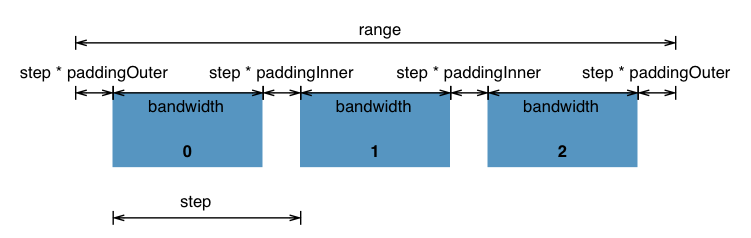 # d3.scaleBand([[domain, ]range]) · Source, Examples
Constructs a new band scale with the specified domain and range, no padding, no rounding and center alignment.
If domain is not specified, it defaults to the empty domain.
If range is not specified, it defaults to the unit range [0, 1].
# band(value) · Source, Examples
Given a value in the input domain, returns the start of the corresponding band derived from the output range.
If the given value is not in the scale’s domain, returns undefined.
# band.domain([domain]) · Source, Examples
If domain is specified, sets the domain to the specified array of values.
The first element in domain will be mapped to the first band, the second domain value to the second band, and so on.
Domain values are stored internally in a map from stringified value to index; the resulting index is then used to determine the band.
Thus, a band scale’s values must be coercible to a string, and the stringified version of the domain value uniquely identifies the corresponding band.
If domain is not specified, this method returns the current domain.
# band.range([range]) · Source, Examples
If range is specified, sets the scale’s range to the specified two-element array of numbers.
If the elements in the given array are not numbers, they will be coerced to numbers.
If range is not specified, returns the scale’s current range, which defaults to [0, 1].
# band.rangeRound([range]) · Source, Examples
Sets the scale’s range to the specified two-element array of numbers while also enabling rounding.
This is a convenience method equivalent to:
band
.range(range)
.round(true);
Rounding is sometimes useful for avoiding antialiasing artifacts, though also consider the shape-rendering “crispEdges” styles.
# band.round([round]) · Source, Examples
If round is specified, enables or disables rounding accordingly.
If rounding is enabled, the start and stop of each band will be integers.
Rounding is sometimes useful for avoiding antialiasing artifacts, though also consider the shape-rendering “crispEdges” styles.
Note that if the width of the domain is not a multiple of the cardinality of the range, there may be leftover unused space, even without padding! Use band.align to specify how the leftover space is distributed.
# band.paddingInner([padding]) · Source, Examples
If padding is specified, sets the inner padding to the specified number which must be less than or equal to 1.
If padding is not specified, returns the current inner padding which defaults to 0.
The inner padding specifies the proportion of the range that is reserved for blank space between bands; a value of 0 means no blank space between bands, and a value of 1 means a bandwidth of zero.
# band.paddingOuter([padding]) · Source, Examples
If padding is specified, sets the outer padding to the specified number which is typically in the range [0, 1].
If padding is not specified, returns the current outer padding which defaults to 0.
The outer padding specifies the amount of blank space, in terms of multiples of the step, to reserve before the first band and after the last band.
# band.padding([padding]) · Source, Examples
A convenience method for setting the inner and outer padding to the same padding value.
If padding is not specified, returns the inner padding.
# band.align([align]) · Source, Examples
If align is specified, sets the alignment to the specified value which must be in the range [0, 1].
If align is not specified, returns the current alignment which defaults to 0.5.
The alignment specifies how outer padding is distributed in the range.
A value of 0.5 indicates that the outer padding should be equally distributed before the first band and after the last band; i.e., the bands should be centered within the range.
A value of 0 or 1 may be used to shift the bands to one side, say to position them adjacent to an axis.
For more, see this explainer.
# band.bandwidth() · Source, Examples
Returns the width of each band.
# band.step() · Source, Examples
Returns the distance between the starts of adjacent bands.
# band.copy() · Source, Examples
Returns an exact copy of this scale.
Changes to this scale will not affect the returned scale, and vice versa.
# d3.scaleBand([[domain, ]range]) · Source, Examples
Constructs a new band scale with the specified domain and range, no padding, no rounding and center alignment.
If domain is not specified, it defaults to the empty domain.
If range is not specified, it defaults to the unit range [0, 1].
# band(value) · Source, Examples
Given a value in the input domain, returns the start of the corresponding band derived from the output range.
If the given value is not in the scale’s domain, returns undefined.
# band.domain([domain]) · Source, Examples
If domain is specified, sets the domain to the specified array of values.
The first element in domain will be mapped to the first band, the second domain value to the second band, and so on.
Domain values are stored internally in a map from stringified value to index; the resulting index is then used to determine the band.
Thus, a band scale’s values must be coercible to a string, and the stringified version of the domain value uniquely identifies the corresponding band.
If domain is not specified, this method returns the current domain.
# band.range([range]) · Source, Examples
If range is specified, sets the scale’s range to the specified two-element array of numbers.
If the elements in the given array are not numbers, they will be coerced to numbers.
If range is not specified, returns the scale’s current range, which defaults to [0, 1].
# band.rangeRound([range]) · Source, Examples
Sets the scale’s range to the specified two-element array of numbers while also enabling rounding.
This is a convenience method equivalent to:
band
.range(range)
.round(true);
Rounding is sometimes useful for avoiding antialiasing artifacts, though also consider the shape-rendering “crispEdges” styles.
# band.round([round]) · Source, Examples
If round is specified, enables or disables rounding accordingly.
If rounding is enabled, the start and stop of each band will be integers.
Rounding is sometimes useful for avoiding antialiasing artifacts, though also consider the shape-rendering “crispEdges” styles.
Note that if the width of the domain is not a multiple of the cardinality of the range, there may be leftover unused space, even without padding! Use band.align to specify how the leftover space is distributed.
# band.paddingInner([padding]) · Source, Examples
If padding is specified, sets the inner padding to the specified number which must be less than or equal to 1.
If padding is not specified, returns the current inner padding which defaults to 0.
The inner padding specifies the proportion of the range that is reserved for blank space between bands; a value of 0 means no blank space between bands, and a value of 1 means a bandwidth of zero.
# band.paddingOuter([padding]) · Source, Examples
If padding is specified, sets the outer padding to the specified number which is typically in the range [0, 1].
If padding is not specified, returns the current outer padding which defaults to 0.
The outer padding specifies the amount of blank space, in terms of multiples of the step, to reserve before the first band and after the last band.
# band.padding([padding]) · Source, Examples
A convenience method for setting the inner and outer padding to the same padding value.
If padding is not specified, returns the inner padding.
# band.align([align]) · Source, Examples
If align is specified, sets the alignment to the specified value which must be in the range [0, 1].
If align is not specified, returns the current alignment which defaults to 0.5.
The alignment specifies how outer padding is distributed in the range.
A value of 0.5 indicates that the outer padding should be equally distributed before the first band and after the last band; i.e., the bands should be centered within the range.
A value of 0 or 1 may be used to shift the bands to one side, say to position them adjacent to an axis.
For more, see this explainer.
# band.bandwidth() · Source, Examples
Returns the width of each band.
# band.step() · Source, Examples
Returns the distance between the starts of adjacent bands.
# band.copy() · Source, Examples
Returns an exact copy of this scale.
Changes to this scale will not affect the returned scale, and vice versa.
Point Scales
Point scales are a variant of band scales with the bandwidth fixed to zero.
Point scales are typically used for scatterplots with an ordinal or categorical dimension.
The unknown value of a point scale is always undefined: they do not allow implicit domain construction.
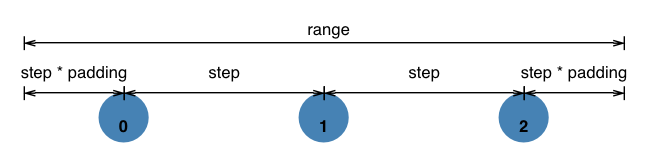 # d3.scalePoint([[domain, ]range]) · Source, Examples
Constructs a new point scale with the specified domain and range, no padding, no rounding and center alignment.
If domain is not specified, it defaults to the empty domain.
If range is not specified, it defaults to the unit range [0, 1].
# point(value) · Source, Examples
Given a value in the input domain, returns the corresponding point derived from the output range.
If the given value is not in the scale’s domain, returns undefined.
# point.domain([domain]) · Source, Examples
If domain is specified, sets the domain to the specified array of values.
The first element in domain will be mapped to the first point, the second domain value to the second point, and so on.
Domain values are stored internally in a map from stringified value to index; the resulting index is then used to determine the point.
Thus, a point scale’s values must be coercible to a string, and the stringified version of the domain value uniquely identifies the corresponding point.
If domain is not specified, this method returns the current domain.
# point.range([range]) · Source, Examples
If range is specified, sets the scale’s range to the specified two-element array of numbers.
If the elements in the given array are not numbers, they will be coerced to numbers.
If range is not specified, returns the scale’s current range, which defaults to [0, 1].
# point.rangeRound([range]) · Source, Examples
Sets the scale’s range to the specified two-element array of numbers while also enabling rounding.
This is a convenience method equivalent to:
point
.range(range)
.round(true);
Rounding is sometimes useful for avoiding antialiasing artifacts, though also consider the shape-rendering “crispEdges” styles.
# point.round([round]) · Source, Examples
If round is specified, enables or disables rounding accordingly.
If rounding is enabled, the position of each point will be integers.
Rounding is sometimes useful for avoiding antialiasing artifacts, though also consider the shape-rendering “crispEdges” styles.
Note that if the width of the domain is not a multiple of the cardinality of the range, there may be leftover unused space, even without padding! Use point.align to specify how the leftover space is distributed.
# point.padding([padding]) · Source, Examples
If padding is specified, sets the outer padding to the specified number which is typically in the range [0, 1].
If padding is not specified, returns the current outer padding which defaults to 0.
The outer padding specifies the amount of blank space, in terms of multiples of the step, to reserve before the first point and after the last point.
Equivalent to band.paddingOuter.
# point.align([align]) · Source, Examples
If align is specified, sets the alignment to the specified value which must be in the range [0, 1].
If align is not specified, returns the current alignment which defaults to 0.5.
The alignment specifies how any leftover unused space in the range is distributed.
A value of 0.5 indicates that the leftover space should be equally distributed before the first point and after the last point; i.e., the points should be centered within the range.
A value of 0 or 1 may be used to shift the points to one side, say to position them adjacent to an axis.
# point.bandwidth() · Source, Examples
Returns zero.
# point.step() · Source, Examples
Returns the distance between the starts of adjacent points.
# point.copy() · Source, Examples
Returns an exact copy of this scale.
Changes to this scale will not affect the returned scale, and vice versa.
# d3.scalePoint([[domain, ]range]) · Source, Examples
Constructs a new point scale with the specified domain and range, no padding, no rounding and center alignment.
If domain is not specified, it defaults to the empty domain.
If range is not specified, it defaults to the unit range [0, 1].
# point(value) · Source, Examples
Given a value in the input domain, returns the corresponding point derived from the output range.
If the given value is not in the scale’s domain, returns undefined.
# point.domain([domain]) · Source, Examples
If domain is specified, sets the domain to the specified array of values.
The first element in domain will be mapped to the first point, the second domain value to the second point, and so on.
Domain values are stored internally in a map from stringified value to index; the resulting index is then used to determine the point.
Thus, a point scale’s values must be coercible to a string, and the stringified version of the domain value uniquely identifies the corresponding point.
If domain is not specified, this method returns the current domain.
# point.range([range]) · Source, Examples
If range is specified, sets the scale’s range to the specified two-element array of numbers.
If the elements in the given array are not numbers, they will be coerced to numbers.
If range is not specified, returns the scale’s current range, which defaults to [0, 1].
# point.rangeRound([range]) · Source, Examples
Sets the scale’s range to the specified two-element array of numbers while also enabling rounding.
This is a convenience method equivalent to:
point
.range(range)
.round(true);
Rounding is sometimes useful for avoiding antialiasing artifacts, though also consider the shape-rendering “crispEdges” styles.
# point.round([round]) · Source, Examples
If round is specified, enables or disables rounding accordingly.
If rounding is enabled, the position of each point will be integers.
Rounding is sometimes useful for avoiding antialiasing artifacts, though also consider the shape-rendering “crispEdges” styles.
Note that if the width of the domain is not a multiple of the cardinality of the range, there may be leftover unused space, even without padding! Use point.align to specify how the leftover space is distributed.
# point.padding([padding]) · Source, Examples
If padding is specified, sets the outer padding to the specified number which is typically in the range [0, 1].
If padding is not specified, returns the current outer padding which defaults to 0.
The outer padding specifies the amount of blank space, in terms of multiples of the step, to reserve before the first point and after the last point.
Equivalent to band.paddingOuter.
# point.align([align]) · Source, Examples
If align is specified, sets the alignment to the specified value which must be in the range [0, 1].
If align is not specified, returns the current alignment which defaults to 0.5.
The alignment specifies how any leftover unused space in the range is distributed.
A value of 0.5 indicates that the leftover space should be equally distributed before the first point and after the last point; i.e., the points should be centered within the range.
A value of 0 or 1 may be used to shift the points to one side, say to position them adjacent to an axis.
# point.bandwidth() · Source, Examples
Returns zero.
# point.step() · Source, Examples
Returns the distance between the starts of adjacent points.
# point.copy() · Source, Examples
Returns an exact copy of this scale.
Changes to this scale will not affect the returned scale, and vice versa.
d3-selection
Selections allow powerful data-driven transformation of the document object model (DOM): set attributes, styles, properties, HTML or text content, and more.
Using the data join’s enter and exit selections, you can also add or remove elements to correspond to data.
Selection methods typically return the current selection, or a new selection, allowing the concise application of multiple operations on a given selection via method chaining.
For example, to set the class and color style of all paragraph elements in the current document:
d3.selectAll("p")
.attr("class", "graf")
.style("color", "red");
This is equivalent to:
const p = d3.selectAll("p");
p.attr("class", "graf");
p.style("color", "red");
By convention, selection methods that return the current selection use four spaces of indent, while methods that return a new selection use only two.
This helps reveal changes of context by making them stick out of the chain:
d3.select("body")
.append("svg")
.attr("width", 960)
.attr("height", 500)
.append("g")
.attr("transform", "translate(20,20)")
.append("rect")
.attr("width", 920)
.attr("height", 460);
Selections are immutable.
All selection methods that affect which elements are selected (or their order) return a new selection rather than modifying the current selection.
However, note that elements are necessarily mutable, as selections drive transformations of the document!
For more, see the d3-selection collection on Observable.
Installing
If you use NPM, npm install d3-selection.
Otherwise, download the latest release.
You can also load d3-selection as a standalone library or as part of D3.
ES modules, AMD, CommonJS, and vanilla environments are supported.
In vanilla, a d3 global is exported:
<script src="https://cdn.jsdelivr.net/npm/d3-selection@2"></script>
<script>
const div = d3.selectAll("div");
</script>
Try d3-selection in your browser.
API Reference
Selecting Elements
Modifying Elements
Joining Data
Handling Events
Control Flow
Local Variables
Namespaces
Selecting Elements
Selection methods accept W3C selector strings such as .fancy to select elements with the class fancy, or div to select DIV elements.
Selection methods come in two forms: select and selectAll: the former selects only the first matching element, while the latter selects all matching elements in document order.
The top-level selection methods, d3.select and d3.selectAll, query the entire document; the subselection methods, selection.select and selection.selectAll, restrict selection to descendants of the selected elements.
# d3.selection() · Source
Selects the root element, document.documentElement.
This function can also be used to test for selections (instanceof d3.selection) or to extend the selection prototype.
For example, to add a method to check checkboxes:
d3.selection.prototype.checked = function(value) {
return arguments.length < 1
? this.property("checked")
: this.property("checked", !!value);
};
And then to use:
d3.selectAll("input[type=checkbox]").checked(true);
# d3.select(selector) · Source
Selects the first element that matches the specified selector string.
If no elements match the selector, returns an empty selection.
If multiple elements match the selector, only the first matching element (in document order) will be selected.
For example, to select the first anchor element:
const anchor = d3.select("a");
If the selector is not a string, instead selects the specified node; this is useful if you already have a reference to a node, such as this within an event listener or a global such as document.body.
For example, to make a clicked paragraph red:
d3.selectAll("p").on("click", function(event) {
d3.select(this).style("color", "red");
});
# d3.selectAll(selector) · Source
Selects all elements that match the specified selector string.
The elements will be selected in document order (top-to-bottom).
If no elements in the document match the selector, or if the selector is null or undefined, returns an empty selection.
For example, to select all paragraphs:
const paragraph = d3.selectAll("p");
If the selector is not a string, instead selects the specified array of nodes; this is useful if you already have a reference to nodes, such as this.childNodes within an event listener or a global such as document.links.
The nodes may instead be an iterable, or a pseudo-array such as a NodeList.
For example, to color all links red:
d3.selectAll(document.links).style("color", "red");
# selection.select(selector) · Source
For each selected element, selects the first descendant element that matches the specified selector string.
If no element matches the specified selector for the current element, the element at the current index will be null in the returned selection.
(If the selector is null, every element in the returned selection will be null, resulting in an empty selection.) If the current element has associated data, this data is propagated to the corresponding selected element.
If multiple elements match the selector, only the first matching element in document order is selected.
For example, to select the first bold element in every paragraph:
const b = d3.selectAll("p").select("b");
If the selector is a function, it is evaluated for each selected element, in order, being passed the current datum (d), the current index (i), and the current group (nodes), with this as the current DOM element (nodes[i]).
It must return an element, or null if there is no matching element.
For example, to select the previous sibling of each paragraph:
const previous = d3.selectAll("p").select(function() {
return this.previousElementSibling;
});
Unlike selection.selectAll, selection.select does not affect grouping: it preserves the existing group structure and indexes, and propagates data (if any) to selected children.
Grouping plays an important role in the data join.
See Nested Selections and How Selections Work for more on this topic.
# selection.selectAll(selector) · Source
For each selected element, selects the descendant elements that match the specified selector string.
The elements in the returned selection are grouped by their corresponding parent node in this selection.
If no element matches the specified selector for the current element, or if the selector is null, the group at the current index will be empty.
The selected elements do not inherit data from this selection; use selection.data to propagate data to children.
For example, to select the bold elements in every paragraph:
const b = d3.selectAll("p").selectAll("b");
If the selector is a function, it is evaluated for each selected element, in order, being passed the current datum (d), the current index (i), and the current group (nodes), with this as the current DOM element (nodes[i]).
It must return an array of elements (or an iterable, or a pseudo-array such as a NodeList), or the empty array if there are no matching elements.
For example, to select the previous and next siblings of each paragraph:
const sibling = d3.selectAll("p").selectAll(function() {
return [
this.previousElementSibling,
this.nextElementSibling
];
});
Unlike selection.select, selection.selectAll does affect grouping: each selected descendant is grouped by the parent element in the originating selection.
Grouping plays an important role in the data join.
See Nested Selections and How Selections Work for more on this topic.
# selection.filter(filter) · Source
Filters the selection, returning a new selection that contains only the elements for which the specified filter is true.
The filter may be specified either as a selector string or a function.
If the filter is a function, it is evaluated for each selected element, in order, being passed the current datum (d), the current index (i), and the current group (nodes), with this as the current DOM element (nodes[i]).
For example, to filter a selection of table rows to contain only even rows:
const even = d3.selectAll("tr").filter(":nth-child(even)");
This is approximately equivalent to using d3.selectAll directly, although the indexes may be different:
const even = d3.selectAll("tr:nth-child(even)");
Similarly, using a function:
const even = d3.selectAll("tr").filter((d, i) => i & 1);
Or using selection.select (and avoiding an arrow function, since this is needed to refer to the current element):
const even = d3.selectAll("tr").select(function(d, i) { return i & 1 ? this : null; });
Note that the :nth-child pseudo-class is a one-based index rather than a zero-based index.
Also, the above filter functions do not have precisely the same meaning as :nth-child; they rely on the selection index rather than the number of preceding sibling elements in the DOM.
The returned filtered selection preserves the parents of this selection, but like array.filter, it does not preserve indexes as some elements may be removed; use selection.select to preserve the index, if needed.
# selection.merge(other) · Source
Returns a new selection merging this selection with the specified other selection.
The returned selection has the same number of groups and the same parents as this selection.
Any missing (null) elements in this selection are filled with the corresponding element, if present (not null), from the specified selection.
(If the other selection has additional groups or parents, they are ignored.)
This method is used internally by selection.join to merge the enter and update selections after binding data.
You can also merge explicitly, although note that since merging is based on element index, you should use operations that preserve index, such as selection.select instead of selection.filter.
For example:
const odd = selection.select(function(d, i) { return i & 1 ? this : null; ));
const even = selection.select(function(d, i) { return i & 1 ? null : this; ));
const merged = odd.merge(even);
See selection.data for more.
This method is not intended for concatenating arbitrary selections, however: if both this selection and the specified other selection have (non-null) elements at the same index, this selection’s element is returned in the merge and the other selection’s element is ignored.
# selection.selectChild([selector]) · Source
Returns a new selection with the (first) child of each element of the current selection matching the selector.
If no selector is specified, selects the first child (if any).
If the selector is specified as a string, selects the first child that matches (if any).
If the selector is a function, it is evaluated for each of the children nodes, in order, being passed the child (child), the child’s index (i), and the list of children (children); the method selects the first child for which the selector return truthy, if any.
# selection.selectChildren([selector]) · Source
Returns a new selection with the children of each element of the current selection matching the selector.
If no selector is specified, selects all the children.
If the selector is specified as a string, selects the children that match (if any).
If the selector is a function, it is evaluated for each of the children nodes, in order, being passed the child (child), the child’s index (i), and the list of children (children); the method selects all children for which the selector return truthy.
# selection.selection() · Source
Returns the selection (for symmetry with transition.selection).
# d3.matcher(selector) · Source
Given the specified selector, returns a function which returns true if this element matches the specified selector.
This method is used internally by selection.filter.
For example, this:
const div = selection.filter("div");
Is equivalent to:
const div = selection.filter(d3.matcher("div"));
(Although D3 is not a compatibility layer, this implementation does support vendor-prefixed implementations due to the recent standardization of element.matches.)
# d3.selector(selector) · Source
Given the specified selector, returns a function which returns the first descendant of this element that matches the specified selector.
This method is used internally by selection.select.
For example, this:
const div = selection.select("div");
Is equivalent to:
const div = selection.select(d3.selector("div"));
# d3.selectorAll(selector) · Source
Given the specified selector, returns a function which returns all descendants of this element that match the specified selector.
This method is used internally by selection.selectAll.
For example, this:
const div = selection.selectAll("div");
Is equivalent to:
const div = selection.selectAll(d3.selectorAll("div"));
# d3.window(node) · Source
Returns the owner window for the specified node.
If node is a node, returns the owner document’s default view; if node is a document, returns its default view; otherwise returns the node.
# d3.style(node, name) · Source
Returns the value of the style property with the specified name for the specified node.
If the node has an inline style with the specified name, its value is returned; otherwise, the computed property value is returned.
See also selection.style.
Modifying Elements
After selecting elements, use the selection’s transformation methods to affect document content.
For example, to set the name attribute and color style of an anchor element:
d3.select("a")
.attr("name", "fred")
.style("color", "red");
To experiment with selections, visit d3js.org and open your browser’s developer console! (In Chrome, open the console with J.) Select elements and then inspect the returned selection to see which elements are selected and how they are grouped.
Call selection methods and see how the page content changes.
# selection.attr(name[, value]) · Source
If a value is specified, sets the attribute with the specified name to the specified value on the selected elements and returns this selection.
If the value is a constant, all elements are given the same attribute value; otherwise, if the value is a function, it is evaluated for each selected element, in order, being passed the current datum (d), the current index (i), and the current group (nodes), with this as the current DOM element (nodes[i]).
The function’s return value is then used to set each element’s attribute.
A null value will remove the specified attribute.
If a value is not specified, returns the current value of the specified attribute for the first (non-null) element in the selection.
This is generally useful only if you know that the selection contains exactly one element.
The specified name may have a namespace prefix, such as xlink:href to specify the href attribute in the XLink namespace.
See namespaces for the map of supported namespaces; additional namespaces can be registered by adding to the map.
# selection.classed(names[, value]) · Source
If a value is specified, assigns or unassigns the specified CSS class names on the selected elements by setting the class attribute or modifying the classList property and returns this selection.
The specified names is a string of space-separated class names.
For example, to assign the classes foo and bar to the selected elements:
selection.classed("foo bar", true);
If the value is truthy, then all elements are assigned the specified classes; otherwise, the classes are unassigned.
If the value is a function, it is evaluated for each selected element, in order, being passed the current datum (d), the current index (i), and the current group (nodes), with this as the current DOM element (nodes[i]).
The function’s return value is then used to assign or unassign classes on each element.
For example, to randomly associate the class foo with on average half the selected elements:
selection.classed("foo", () => Math.random() > 0.5);
If a value is not specified, returns true if and only if the first (non-null) selected element has the specified classes.
This is generally useful only if you know the selection contains exactly one element.
# selection.style(name[, value[, priority]]) · Source
If a value is specified, sets the style property with the specified name to the specified value on the selected elements and returns this selection.
If the value is a constant, then all elements are given the same style property value; otherwise, if the value is a function, it is evaluated for each selected element, in order, being passed the current datum (d), the current index (i), and the current group (nodes), with this as the current DOM element (nodes[i]).
The function’s return value is then used to set each element’s style property.
A null value will remove the style property.
An optional priority may also be specified, either as null or the string important (without the exclamation point).
If a value is not specified, returns the current value of the specified style property for the first (non-null) element in the selection.
The current value is defined as the element’s inline value, if present, and otherwise its computed value.
Accessing the current style value is generally useful only if you know the selection contains exactly one element.
Caution: unlike many SVG attributes, CSS styles typically have associated units.
For example, 3px is a valid stroke-width property value, while 3 is not.
Some browsers implicitly assign the px (pixel) unit to numeric values, but not all browsers do: IE, for example, throws an “invalid arguments” error!
# selection.property(name[, value]) · Source
Some HTML elements have special properties that are not addressable using attributes or styles, such as a form field’s text value and a checkbox’s checked boolean.
Use this method to get or set these properties.
If a value is specified, sets the property with the specified name to the specified value on selected elements.
If the value is a constant, then all elements are given the same property value; otherwise, if the value is a function, it is evaluated for each selected element, in order, being passed the current datum (d), the current index (i), and the current group (nodes), with this as the current DOM element (nodes[i]).
The function’s return value is then used to set each element’s property.
A null value will delete the specified property.
If a value is not specified, returns the value of the specified property for the first (non-null) element in the selection.
This is generally useful only if you know the selection contains exactly one element.
# selection.text([value]) · Source
If a value is specified, sets the text content to the specified value on all selected elements, replacing any existing child elements.
If the value is a constant, then all elements are given the same text content; otherwise, if the value is a function, it is evaluated for each selected element, in order, being passed the current datum (d), the current index (i), and the current group (nodes), with this as the current DOM element (nodes[i]).
The function’s return value is then used to set each element’s text content.
A null value will clear the content.
If a value is not specified, returns the text content for the first (non-null) element in the selection.
This is generally useful only if you know the selection contains exactly one element.
# selection.html([value]) · Source
If a value is specified, sets the inner HTML to the specified value on all selected elements, replacing any existing child elements.
If the value is a constant, then all elements are given the same inner HTML; otherwise, if the value is a function, it is evaluated for each selected element, in order, being passed the current datum (d), the current index (i), and the current group (nodes), with this as the current DOM element (nodes[i]).
The function’s return value is then used to set each element’s inner HTML.
A null value will clear the content.
If a value is not specified, returns the inner HTML for the first (non-null) element in the selection.
This is generally useful only if you know the selection contains exactly one element.
Use selection.append or selection.insert instead to create data-driven content; this method is intended for when you want a little bit of HTML, say for rich formatting.
Also, selection.html is only supported on HTML elements.
SVG elements and other non-HTML elements do not support the innerHTML property, and thus are incompatible with selection.html.
Consider using XMLSerializer to convert a DOM subtree to text.
See also the innersvg polyfill, which provides a shim to support the innerHTML property on SVG elements.
# selection.append(type) · Source
If the specified type is a string, appends a new element of this type (tag name) as the last child of each selected element, or before the next following sibling in the update selection if this is an enter selection.
The latter behavior for enter selections allows you to insert elements into the DOM in an order consistent with the new bound data; however, note that selection.order may still be required if updating elements change order (i.e., if the order of new data is inconsistent with old data).
If the specified type is a function, it is evaluated for each selected element, in order, being passed the current datum (d), the current index (i), and the current group (nodes), with this as the current DOM element (nodes[i]).
This function should return an element to be appended.
(The function typically creates a new element, but it may instead return an existing element.) For example, to append a paragraph to each DIV element:
d3.selectAll("div").append("p");
This is equivalent to:
d3.selectAll("div").append(() => document.createElement("p"));
Which is equivalent to:
d3.selectAll("div").select(function() {
return this.appendChild(document.createElement("p"));
});
In both cases, this method returns a new selection containing the appended elements.
Each new element inherits the data of the current elements, if any, in the same manner as selection.select.
The specified name may have a namespace prefix, such as svg:text to specify a text attribute in the SVG namespace.
See namespaces for the map of supported namespaces; additional namespaces can be registered by adding to the map.
If no namespace is specified, the namespace will be inherited from the parent element; or, if the name is one of the known prefixes, the corresponding namespace will be used (for example, svg implies svg:svg).
# selection.insert(type[, before]) · Source
If the specified type is a string, inserts a new element of this type (tag name) before the first element matching the specified before selector for each selected element.
For example, a before selector :first-child will prepend nodes before the first child.
If before is not specified, it defaults to null.
(To append elements in an order consistent with bound data, use selection.append.)
Both type and before may instead be specified as functions which are evaluated for each selected element, in order, being passed the current datum (d), the current index (i), and the current group (nodes), with this as the current DOM element (nodes[i]).
The type function should return an element to be inserted; the before function should return the child element before which the element should be inserted.
For example, to append a paragraph to each DIV element:
d3.selectAll("div").insert("p");
This is equivalent to:
d3.selectAll("div").insert(() => document.createElement("p"));
Which is equivalent to:
d3.selectAll("div").select(function() {
return this.insertBefore(document.createElement("p"), null);
});
In both cases, this method returns a new selection containing the appended elements.
Each new element inherits the data of the current elements, if any, in the same manner as selection.select.
The specified name may have a namespace prefix, such as svg:text to specify a text attribute in the SVG namespace.
See namespaces for the map of supported namespaces; additional namespaces can be registered by adding to the map.
If no namespace is specified, the namespace will be inherited from the parent element; or, if the name is one of the known prefixes, the corresponding namespace will be used (for example, svg implies svg:svg).
# selection.remove() · Source
Removes the selected elements from the document.
Returns this selection (the removed elements) which are now detached from the DOM.
There is not currently a dedicated API to add removed elements back to the document; however, you can pass a function to selection.append or selection.insert to re-add elements.
# selection.clone([deep]) · Source
Inserts clones of the selected elements immediately following the selected elements and returns a selection of the newly added clones.
If deep is truthy, the descendant nodes of the selected elements will be cloned as well.
Otherwise, only the elements themselves will be cloned.
Equivalent to:
selection.select(function() {
return this.parentNode.insertBefore(this.cloneNode(deep), this.nextSibling);
});
# selection.sort(compare) · Source
Returns a new selection that contains a copy of each group in this selection sorted according to the compare function.
After sorting, re-inserts elements to match the resulting order (per selection.order).
The compare function, which defaults to ascending, is passed two elements’ data a and b to compare.
It should return either a negative, positive, or zero value.
If negative, then a should be before b; if positive, then a should be after b; otherwise, a and b are considered equal and the order is arbitrary.
Note that sorting is not guaranteed to be stable; however, it is guaranteed to have the same behavior as your browser’s built-in sort method on arrays.
# selection.order() · Source
Re-inserts elements into the document such that the document order of each group matches the selection order.
This is equivalent to calling selection.sort if the data is already sorted, but much faster.
# selection.raise() · Source
Re-inserts each selected element, in order, as the last child of its parent.
Equivalent to:
selection.each(function() {
this.parentNode.appendChild(this);
});
# selection.lower() · Source
Re-inserts each selected element, in order, as the first child of its parent.
Equivalent to:
selection.each(function() {
this.parentNode.insertBefore(this, this.parentNode.firstChild);
});
# d3.create(name) · Source
Given the specified element name, returns a single-element selection containing a detached element of the given name in the current document.
This method assumes the HTML namespace, so you must specify a namespace explicitly when creating SVG or other non-HTML elements; see namespace for details on supported namespace prefixes.
d3.create("svg") // equivalent to svg:svg
d3.create("svg:svg") // more explicitly
d3.create("svg:g") // an SVG G element
d3.create("g") // an HTML G (unknown) element
# d3.creator(name) · Source
Given the specified element name, returns a function which creates an element of the given name, assuming that this is the parent element.
This method is used internally by selection.append and selection.insert to create new elements.
For example, this:
selection.append("div");
Is equivalent to:
selection.append(d3.creator("div"));
See namespace for details on supported namespace prefixes, such as for SVG elements.
Joining Data
For an introduction to D3’s data joins, see the selection.join notebook.
Also see Thinking With Joins.
# selection.data([data[, key]]) · Source
Binds the specified array of data with the selected elements, returning a new selection that represents the update selection: the elements successfully bound to data.
Also defines the enter and exit selections on the returned selection, which can be used to add or remove elements to correspond to the new data.
The specified data is an array of arbitrary values (e.g., numbers or objects), or a function that returns an array of values for each group.
When data is assigned to an element, it is stored in the property __data__, thus making the data “sticky” and available on re-selection.
The data is specified for each group in the selection.
If the selection has multiple groups (such as d3.selectAll followed by selection.selectAll), then data should typically be specified as a function.
This function will be evaluated for each group in order, being passed the group’s parent datum (d, which may be undefined), the group index (i), and the selection’s parent nodes (nodes), with this as the group’s parent element.
In conjunction with selection.join (or more explicitly with selection.enter, selection.exit, selection.append and selection.remove), selection.data can be used to enter, update and exit elements to match data.
For example, to create an HTML table from a matrix of numbers:
const matrix = [
[11975, 5871, 8916, 2868],
[ 1951, 10048, 2060, 6171],
[ 8010, 16145, 8090, 8045],
[ 1013, 990, 940, 6907]
];
d3.select("body")
.append("table")
.selectAll("tr")
.data(matrix)
.join("tr")
.selectAll("td")
.data(d => d)
.join("td")
.text(d => d);
In this example the data function is the identity function: for each table row, it returns the corresponding row from the data matrix.
If a key function is not specified, then the first datum in data is assigned to the first selected element, the second datum to the second selected element, and so on.
A key function may be specified to control which datum is assigned to which element, replacing the default join-by-index, by computing a string identifier for each datum and element.
This key function is evaluated for each selected element, in order, being passed the current datum (d), the current index (i), and the current group (nodes), with this as the current DOM element (nodes[i]); the returned string is the element’s key.
The key function is then also evaluated for each new datum in data, being passed the current datum (d), the current index (i), and the group’s new data, with this as the group’s parent DOM element; the returned string is the datum’s key.
The datum for a given key is assigned to the element with the matching key.
If multiple elements have the same key, the duplicate elements are put into the exit selection; if multiple data have the same key, the duplicate data are put into the enter selection.
For example, given this document:
<div id="Ford"></div>
<div id="Jarrah"></div>
<div id="Kwon"></div>
<div id="Locke"></div>
<div id="Reyes"></div>
<div id="Shephard"></div>
You could join data by key as follows:
const data = [
{name: "Locke", number: 4},
{name: "Reyes", number: 8},
{name: "Ford", number: 15},
{name: "Jarrah", number: 16},
{name: "Shephard", number: 23},
{name: "Kwon", number: 42}
];
d3.selectAll("div")
.data(data, function(d) { return d ? d.name : this.id; })
.text(d => d.number);
This example key function uses the datum d if present, and otherwise falls back to the element’s id property.
Since these elements were not previously bound to data, the datum d is null when the key function is evaluated on selected elements, and non-null when the key function is evaluated on the new data.
The update and enter selections are returned in data order, while the exit selection preserves the selection order prior to the join.
If a key function is specified, the order of elements in the selection may not match their order in the document; use selection.order or selection.sort as needed.
For more on how the key function affects the join, see A Bar Chart, Part 2 and Object Constancy.
If data is not specified, this method returns the array of data for the selected elements.
This method cannot be used to clear bound data; use selection.datum instead.
# selection.join(enter[, update][, exit]) · Source
Appends, removes and reorders elements as necessary to match the data that was previously bound by selection.data, returning the merged enter and update selection.
This method is a convenient alternative to the explicit general update pattern, replacing selection.enter, selection.exit, selection.append, selection.remove, and selection.order.
For example:
svg.selectAll("circle")
.data(data)
.join("circle")
.attr("fill", "none")
.attr("stroke", "black");
The enter function may be specified as a string shorthand, as above, which is equivalent to selection.append with the given element name.
Likewise, optional update and exit functions may be specified, which default to the identity function and calling selection.remove, respectively.
The shorthand above is thus equivalent to:
svg.selectAll("circle")
.data(data)
.join(
enter => enter.append("circle"),
update => update,
exit => exit.remove()
)
.attr("fill", "none")
.attr("stroke", "black");
By passing separate functions on enter, update and exit, you have greater control over what happens.
And by specifying a key function to selection.data, you can minimize changes to the DOM to optimize performance.
For example, to set different fill colors for enter and update:
svg.selectAll("circle")
.data(data)
.join(
enter => enter.append("circle").attr("fill", "green"),
update => update.attr("fill", "blue")
)
.attr("stroke", "black");
The selections returned by the enter and update functions are merged and then returned by selection.join.
You also animate enter, update and exit by creating transitions inside the enter, update and exit functions.
To avoid breaking the method chain, use selection.call to create transitions, or return an undefined enter or update selection to prevent merging: the return value of the enter and update functions specifies the two selections to merge and return by selection.join.
For more, see the selection.join notebook.
# selection.enter() · Source
Returns the enter selection: placeholder nodes for each datum that had no corresponding DOM element in the selection.
(The enter selection is empty for selections not returned by selection.data.)
The enter selection is typically used to create “missing” elements corresponding to new data.
For example, to create DIV elements from an array of numbers:
const div = d3.select("body")
.selectAll("div")
.data([4, 8, 15, 16, 23, 42])
.enter().append("div")
.text(d => d);
If the body is initially empty, the above code will create six new DIV elements, append them to the body in-order, and assign their text content as the associated (string-coerced) number:
<div>4</div>
<div>8</div>
<div>15</div>
<div>16</div>
<div>23</div>
<div>42</div>
Conceptually, the enter selection’s placeholders are pointers to the parent element (in this example, the document body).
The enter selection is typically only used transiently to append elements, and is often merged with the update selection after appending, such that modifications can be applied to both entering and updating elements.
# selection.exit() · Source
Returns the exit selection: existing DOM elements in the selection for which no new datum was found.
(The exit selection is empty for selections not returned by selection.data.)
The exit selection is typically used to remove “superfluous” elements corresponding to old data.
For example, to update the DIV elements created previously with a new array of numbers:
div = div.data([1, 2, 4, 8, 16, 32], d => d);
Since a key function was specified (as the identity function), and the new data contains the numbers [4, 8, 16] which match existing elements in the document, the update selection contains three DIV elements.
Leaving those elements as-is, we can append new elements for [1, 2, 32] using the enter selection:
div.enter().append("div").text(d => d);
Likewise, to remove the exiting elements [15, 23, 42]:
div.exit().remove();
Now the document body looks like this:
<div>1</div>
<div>2</div>
<div>4</div>
<div>8</div>
<div>16</div>
<div>32</div>
The order of the DOM elements matches the order of the data because the old data’s order and the new data’s order were consistent.
If the new data’s order is different, use selection.order to reorder the elements in the DOM.
See the General Update Pattern example thread for more on data joins.
# selection.datum([value]) · Source
Gets or sets the bound data for each selected element.
Unlike selection.data, this method does not compute a join and does not affect indexes or the enter and exit selections.
If a value is specified, sets the element’s bound data to the specified value on all selected elements.
If the value is a constant, all elements are given the same datum; otherwise, if the value is a function, it is evaluated for each selected element, in order, being passed the current datum (d), the current index (i), and the current group (nodes), with this as the current DOM element (nodes[i]).
The function is then used to set each element’s new data.
A null value will delete the bound data.
If a value is not specified, returns the bound datum for the first (non-null) element in the selection.
This is generally useful only if you know the selection contains exactly one element.
This method is useful for accessing HTML5 custom data attributes.
For example, given the following elements:
<ul id="list">
<li data-username="shawnbot">Shawn Allen</li>
<li data-username="mbostock">Mike Bostock</li>
</ul>
You can expose the custom data attributes by setting each element’s data as the built-in dataset property:
selection.datum(function() { return this.dataset; })
Handling Events
For interaction, selections allow listening for and dispatching of events.
# selection.on(typenames[, listener[, options]]) · Source
Adds or removes a listener to each selected element for the specified event typenames.
The typenames is a string event type, such as click, mouseover, or submit; any DOM event type supported by your browser may be used.
The type may be optionally followed by a period (.) and a name; the optional name allows multiple callbacks to be registered to receive events of the same type, such as click.foo and click.bar.
To specify multiple typenames, separate typenames with spaces, such as input change or click.foo click.bar.
When a specified event is dispatched on a selected element, the specified listener will be evaluated for the element, being passed the current event (event) and the current datum (d), with this as the current DOM element (event.currentTarget).
Listeners always see the latest datum for their element.
Note: while you can use event.pageX and event.pageY directly, it is often convenient to transform the event position to the local coordinate system of the element that received the event using d3.pointer.
If an event listener was previously registered for the same typename on a selected element, the old listener is removed before the new listener is added.
To remove a listener, pass null as the listener.
To remove all listeners for a given name, pass null as the listener and .foo as the typename, where foo is the name; to remove all listeners with no name, specify . as the typename.
An optional options object may specify characteristics about the event listener, such as whether it is capturing or passive; see element.addEventListener.
If a listener is not specified, returns the currently-assigned listener for the specified event typename on the first (non-null) selected element, if any.
If multiple typenames are specified, the first matching listener is returned.
# selection.dispatch(type[, parameters]) · Source
Dispatches a custom event of the specified type to each selected element, in order.
An optional parameters map may be specified to set additional properties of the event.
It may contain the following fields:
bubbles - if true, the event is dispatched to ancestors in reverse tree order.
cancelable - if true, event.preventDefault is allowed.
detail - any custom data associated with the event.
If parameters is a function, it is evaluated for each selected element, in order, being passed the current datum (d), the current index (i), and the current group (nodes), with this as the current DOM element (nodes[i]).
It must return the parameters map for the current element.
# d3.pointer(event[, target]) · Source
Returns a two-element array of numbers [x, y] representing the coordinates of the specified event relative to the specified target.
event can be a UIEvent (MouseEvent or TouchEvent), a PointerEvent, a custom event holding a UIEvent as event.sourceEvent, or a touch.
If target is not specified, it defaults to the source event’s currentTarget property, if available.
If the target is an SVG element, the event’s coordinates are transformed using the inverse of the screen coordinate transformation matrix.
If the target is an HTML element, the event’s coordinates are translated relative to the top-left corner of the target’s bounding client rectangle.
(As such, the coordinate system can only be translated relative to the client coordinates.
See also GeometryUtils.)
Otherwise, [event.pageX, event.pageY] is returned.
In the case of touch events, the coordinates of the first touch are returned.
To handle multitouch interactions, see pointers instead.
# d3.pointers(event[, target]) · Source
Returns an array [[x0, y0], [x1, y1]…] of coordinates of the specified event’s pointer locations relative to the specified target.
For mouse, stylus or single touch events, [x0, y0] is equivalent to d3.pointer(event, target).
In the case of multi-touch events, the returned array contains a pair of coordinates for each of the touches.
If target is not specified, it defaults to the source event’s currentTarget property, if available.
Control Flow
For advanced usage, selections provide methods for custom control flow.
# selection.each(function) · Source
Invokes the specified function for each selected element, in order, being passed the current datum (d), the current index (i), and the current group (nodes), with this as the current DOM element (nodes[i]).
This method can be used to invoke arbitrary code for each selected element, and is useful for creating a context to access parent and child data simultaneously, such as:
parent.each(function(p, j) {
d3.select(this)
.selectAll(".child")
.text(d => `child ${d.name} of ${p.name}`);
});
See Sized Donut Multiples for an example.
# selection.call(function[, arguments…]) · Source
Invokes the specified function exactly once, passing in this selection along with any optional arguments.
Returns this selection.
This is equivalent to invoking the function by hand but facilitates method chaining.
For example, to set several styles in a reusable function:
function name(selection, first, last) {
selection
.attr("first-name", first)
.attr("last-name", last);
}
Now say:
d3.selectAll("div").call(name, "John", "Snow");
This is roughly equivalent to:
name(d3.selectAll("div"), "John", "Snow");
The only difference is that selection.call always returns the selection and not the return value of the called function, name.
# selection.empty() · Source
Returns true if this selection contains no (non-null) elements.
# selection.nodes() · Source
Returns an array of all (non-null) elements in this selection.
Equivalent to:
const elements = Array.from(selection);
See also selection[Symbol.iterator].
# selection.node() · Source
Returns the first (non-null) element in this selection.
If the selection is empty, returns null.
# selection.size() · Source
Returns the total number of (non-null) elements in this selection.
# selectionSymbol.iterator · Source
Returns an iterator over the selected (non-null) elements.
For example, to iterate over the selected elements:
for (const element of selection) {
console.log(element);
}
To flatten the selection to an array:
const elements = [...selection];
Local Variables
D3 locals allow you to define local state independent of data.
For instance, when rendering small multiples of time-series data, you might want the same x-scale for all charts but distinct y-scales to compare the relative performance of each metric.
D3 locals are scoped by DOM elements: on set, the value is stored on the given element; on get, the value is retrieved from given element or the nearest ancestor that defines it.
# d3.local() · Source
Declares a new local variable.
For example:
const foo = d3.local();
Like var, each local is a distinct symbolic reference; unlike var, the value of each local is also scoped by the DOM.
# local.set(node, value) · Source
Sets the value of this local on the specified node to the value, and returns the specified value.
This is often performed using selection.each:
selection.each(function(d) { foo.set(this, d.value); });
If you are just setting a single variable, consider using selection.property:
selection.property(foo, d => d.value);
# local.get(node) · Source
Returns the value of this local on the specified node.
If the node does not define this local, returns the value from the nearest ancestor that defines it.
Returns undefined if no ancestor defines this local.
# local.remove(node) · Source
Deletes this local’s value from the specified node.
Returns true if the node defined this local prior to removal, and false otherwise.
If ancestors also define this local, those definitions are unaffected, and thus local.get will still return the inherited value.
# local.toString() · Source
Returns the automatically-generated identifier for this local.
This is the name of the property that is used to store the local’s value on elements, and thus you can also set or get the local’s value using element[local] or by using selection.property.
Namespaces
XML namespaces are fun! Right? Fortunately you can mostly ignore them.
# d3.namespace(name) · Source
Qualifies the specified name, which may or may not have a namespace prefix.
If the name contains a colon (:), the substring before the colon is interpreted as the namespace prefix, which must be registered in d3.namespaces.
Returns an object space and local attributes describing the full namespace URL and the local name.
For example:
d3.namespace("svg:text"); // {space: "http://www.w3.org/2000/svg", local: "text"}
If the name does not contain a colon, this function merely returns the input name.
# d3.namespaces · Source
The map of registered namespace prefixes.
The initial value is:
{
svg: "http://www.w3.org/2000/svg",
xhtml: "http://www.w3.org/1999/xhtml",
xlink: "http://www.w3.org/1999/xlink",
xml: "http://www.w3.org/XML/1998/namespace",
xmlns: "http://www.w3.org/2000/xmlns/"
}
Additional prefixes may be assigned as needed to create elements or attributes in other namespaces.
d3-shape
Visualizations typically consist of discrete graphical marks, such as symbols, arcs, lines and areas.
While the rectangles of a bar chart may be easy enough to generate directly using SVG or Canvas, other shapes are complex, such as rounded annular sectors and centripetal Catmull–Rom splines.
This module provides a variety of shape generators for your convenience.
As with other aspects of D3, these shapes are driven by data: each shape generator exposes accessors that control how the input data are mapped to a visual representation.
For example, you might define a line generator for a time series by scaling fields of your data to fit the chart:
var line = d3.line()
.x(function(d) { return x(d.date); })
.y(function(d) { return y(d.value); });
This line generator can then be used to compute the d attribute of an SVG path element:
path.datum(data).attr("d", line);
Or you can use it to render to a Canvas 2D context:
line.context(context)(data);
For more, read Introducing d3-shape.
Installing
If you use NPM, npm install d3-shape.
Otherwise, download the latest release.
You can also load directly from d3js.org, either as a standalone library or as part of D3.
AMD, CommonJS, and vanilla environments are supported.
In vanilla, a d3 global is exported:
<script src="https://d3js.org/d3-path.v2.min.js"></script>
<script src="https://d3js.org/d3-shape.v2.min.js"></script>
<script>
var line = d3.line();
</script>
API Reference
Arcs
Pies
Lines
Areas
Curves
Custom Curves
Links
Symbols
Custom Symbol Types
Stacks
Note: all the methods that accept arrays also accept iterables and convert them to arrays internally.
Arcs
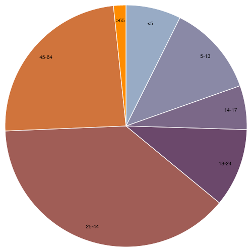
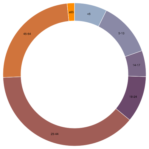 The arc generator produces a circular or annular sector, as in a pie or donut chart.
If the difference between the start and end angles (the angular span) is greater than t, the arc generator will produce a complete circle or annulus.
If it is less than t, arcs may have rounded corners and angular padding.
Arcs are always centered at 0,0; use a transform (see: SVG, Canvas) to move the arc to a different position.
See also the pie generator, which computes the necessary angles to represent an array of data as a pie or donut chart; these angles can then be passed to an arc generator.
# d3.arc() · Source
Constructs a new arc generator with the default settings.
# arc(arguments…) · Source
Generates an arc for the given arguments.
The arguments are arbitrary; they are simply propagated to the arc generator’s accessor functions along with the
The arc generator produces a circular or annular sector, as in a pie or donut chart.
If the difference between the start and end angles (the angular span) is greater than t, the arc generator will produce a complete circle or annulus.
If it is less than t, arcs may have rounded corners and angular padding.
Arcs are always centered at 0,0; use a transform (see: SVG, Canvas) to move the arc to a different position.
See also the pie generator, which computes the necessary angles to represent an array of data as a pie or donut chart; these angles can then be passed to an arc generator.
# d3.arc() · Source
Constructs a new arc generator with the default settings.
# arc(arguments…) · Source
Generates an arc for the given arguments.
The arguments are arbitrary; they are simply propagated to the arc generator’s accessor functions along with the this object.
For example, with the default settings, an object with radii and angles is expected:
var arc = d3.arc();
arc({
innerRadius: 0,
outerRadius: 100,
startAngle: 0,
endAngle: Math.PI / 2
}); // "M0,-100A100,100,0,0,1,100,0L0,0Z"
If the radii and angles are instead defined as constants, you can generate an arc without any arguments:
var arc = d3.arc()
.innerRadius(0)
.outerRadius(100)
.startAngle(0)
.endAngle(Math.PI / 2);
arc(); // "M0,-100A100,100,0,0,1,100,0L0,0Z"
If the arc generator has a context, then the arc is rendered to this context as a sequence of path method calls and this function returns void.
Otherwise, a path data string is returned.
# arc.centroid(arguments…) · Source
Computes the midpoint [x, y] of the center line of the arc that would be generated by the given arguments.
The arguments are arbitrary; they are simply propagated to the arc generator’s accessor functions along with the this object.
To be consistent with the generated arc, the accessors must be deterministic, i.e., return the same value given the same arguments.
The midpoint is defined as (startAngle + endAngle) / 2 and (innerRadius + outerRadius) / 2.
For example:
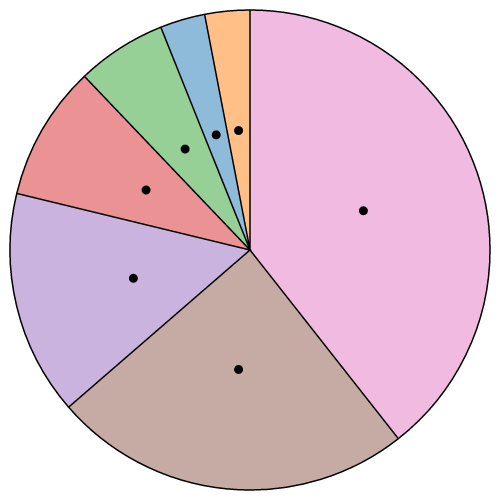
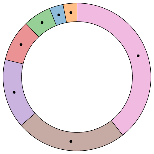 Note that this is not the geometric center of the arc, which may be outside the arc; this method is merely a convenience for positioning labels.
# arc.innerRadius([radius]) · Source
If radius is specified, sets the inner radius to the specified function or number and returns this arc generator.
If radius is not specified, returns the current inner radius accessor, which defaults to:
function innerRadius(d) {
return d.innerRadius;
}
Specifying the inner radius as a function is useful for constructing a stacked polar bar chart, often in conjunction with a sqrt scale.
More commonly, a constant inner radius is used for a donut or pie chart.
If the outer radius is smaller than the inner radius, the inner and outer radii are swapped.
A negative value is treated as zero.
# arc.outerRadius([radius]) · Source
If radius is specified, sets the outer radius to the specified function or number and returns this arc generator.
If radius is not specified, returns the current outer radius accessor, which defaults to:
function outerRadius(d) {
return d.outerRadius;
}
Specifying the outer radius as a function is useful for constructing a coxcomb or polar bar chart, often in conjunction with a sqrt scale.
More commonly, a constant outer radius is used for a pie or donut chart.
If the outer radius is smaller than the inner radius, the inner and outer radii are swapped.
A negative value is treated as zero.
# arc.cornerRadius([radius]) · Source
If radius is specified, sets the corner radius to the specified function or number and returns this arc generator.
If radius is not specified, returns the current corner radius accessor, which defaults to:
function cornerRadius() {
return 0;
}
If the corner radius is greater than zero, the corners of the arc are rounded using circles of the given radius.
For a circular sector, the two outer corners are rounded; for an annular sector, all four corners are rounded.
The corner circles are shown in this diagram:
Note that this is not the geometric center of the arc, which may be outside the arc; this method is merely a convenience for positioning labels.
# arc.innerRadius([radius]) · Source
If radius is specified, sets the inner radius to the specified function or number and returns this arc generator.
If radius is not specified, returns the current inner radius accessor, which defaults to:
function innerRadius(d) {
return d.innerRadius;
}
Specifying the inner radius as a function is useful for constructing a stacked polar bar chart, often in conjunction with a sqrt scale.
More commonly, a constant inner radius is used for a donut or pie chart.
If the outer radius is smaller than the inner radius, the inner and outer radii are swapped.
A negative value is treated as zero.
# arc.outerRadius([radius]) · Source
If radius is specified, sets the outer radius to the specified function or number and returns this arc generator.
If radius is not specified, returns the current outer radius accessor, which defaults to:
function outerRadius(d) {
return d.outerRadius;
}
Specifying the outer radius as a function is useful for constructing a coxcomb or polar bar chart, often in conjunction with a sqrt scale.
More commonly, a constant outer radius is used for a pie or donut chart.
If the outer radius is smaller than the inner radius, the inner and outer radii are swapped.
A negative value is treated as zero.
# arc.cornerRadius([radius]) · Source
If radius is specified, sets the corner radius to the specified function or number and returns this arc generator.
If radius is not specified, returns the current corner radius accessor, which defaults to:
function cornerRadius() {
return 0;
}
If the corner radius is greater than zero, the corners of the arc are rounded using circles of the given radius.
For a circular sector, the two outer corners are rounded; for an annular sector, all four corners are rounded.
The corner circles are shown in this diagram:
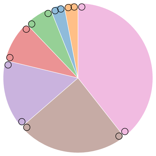
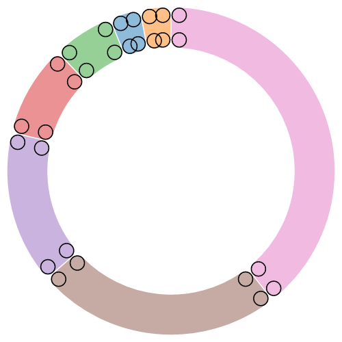 The corner radius may not be larger than (outerRadius - innerRadius) / 2.
In addition, for arcs whose angular span is less than p, the corner radius may be reduced as two adjacent rounded corners intersect.
This is occurs more often with the inner corners.
See the arc corners animation for illustration.
# arc.startAngle([angle]) · Source
If angle is specified, sets the start angle to the specified function or number and returns this arc generator.
If angle is not specified, returns the current start angle accessor, which defaults to:
function startAngle(d) {
return d.startAngle;
}
The angle is specified in radians, with 0 at -y (12 o’clock) and positive angles proceeding clockwise.
If |endAngle - startAngle| = t, a complete circle or annulus is generated rather than a sector.
# arc.endAngle([angle]) · Source
If angle is specified, sets the end angle to the specified function or number and returns this arc generator.
If angle is not specified, returns the current end angle accessor, which defaults to:
function endAngle(d) {
return d.endAngle;
}
The angle is specified in radians, with 0 at -y (12 o’clock) and positive angles proceeding clockwise.
If |endAngle - startAngle| = t, a complete circle or annulus is generated rather than a sector.
# arc.padAngle([angle]) · Source
If angle is specified, sets the pad angle to the specified function or number and returns this arc generator.
If angle is not specified, returns the current pad angle accessor, which defaults to:
function padAngle() {
return d && d.padAngle;
}
The pad angle is converted to a fixed linear distance separating adjacent arcs, defined as padRadius * padAngle.
This distance is subtracted equally from the start and end of the arc.
If the arc forms a complete circle or annulus, as when |endAngle - startAngle| = t, the pad angle is ignored.
If the inner radius or angular span is small relative to the pad angle, it may not be possible to maintain parallel edges between adjacent arcs.
In this case, the inner edge of the arc may collapse to a point, similar to a circular sector.
For this reason, padding is typically only applied to annular sectors (i.e., when innerRadius is positive), as shown in this diagram:
The corner radius may not be larger than (outerRadius - innerRadius) / 2.
In addition, for arcs whose angular span is less than p, the corner radius may be reduced as two adjacent rounded corners intersect.
This is occurs more often with the inner corners.
See the arc corners animation for illustration.
# arc.startAngle([angle]) · Source
If angle is specified, sets the start angle to the specified function or number and returns this arc generator.
If angle is not specified, returns the current start angle accessor, which defaults to:
function startAngle(d) {
return d.startAngle;
}
The angle is specified in radians, with 0 at -y (12 o’clock) and positive angles proceeding clockwise.
If |endAngle - startAngle| = t, a complete circle or annulus is generated rather than a sector.
# arc.endAngle([angle]) · Source
If angle is specified, sets the end angle to the specified function or number and returns this arc generator.
If angle is not specified, returns the current end angle accessor, which defaults to:
function endAngle(d) {
return d.endAngle;
}
The angle is specified in radians, with 0 at -y (12 o’clock) and positive angles proceeding clockwise.
If |endAngle - startAngle| = t, a complete circle or annulus is generated rather than a sector.
# arc.padAngle([angle]) · Source
If angle is specified, sets the pad angle to the specified function or number and returns this arc generator.
If angle is not specified, returns the current pad angle accessor, which defaults to:
function padAngle() {
return d && d.padAngle;
}
The pad angle is converted to a fixed linear distance separating adjacent arcs, defined as padRadius * padAngle.
This distance is subtracted equally from the start and end of the arc.
If the arc forms a complete circle or annulus, as when |endAngle - startAngle| = t, the pad angle is ignored.
If the inner radius or angular span is small relative to the pad angle, it may not be possible to maintain parallel edges between adjacent arcs.
In this case, the inner edge of the arc may collapse to a point, similar to a circular sector.
For this reason, padding is typically only applied to annular sectors (i.e., when innerRadius is positive), as shown in this diagram:
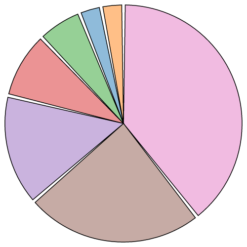
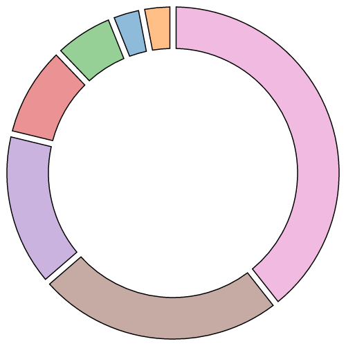 The recommended minimum inner radius when using padding is outerRadius * padAngle / sin, where is the angular span of the smallest arc before padding.
For example, if the outer radius is 200 pixels and the pad angle is 0.02 radians, a reasonable is 0.04 radians, and a reasonable inner radius is 100 pixels.
See the arc padding animation for illustration.
Often, the pad angle is not set directly on the arc generator, but is instead computed by the pie generator so as to ensure that the area of padded arcs is proportional to their value; see pie.padAngle.
See the pie padding animation for illustration.
If you apply a constant pad angle to the arc generator directly, it tends to subtract disproportionately from smaller arcs, introducing distortion.
# arc.padRadius([radius]) · Source
If radius is specified, sets the pad radius to the specified function or number and returns this arc generator.
If radius is not specified, returns the current pad radius accessor, which defaults to null, indicating that the pad radius should be automatically computed as sqrt(innerRadius * innerRadius + outerRadius * outerRadius).
The pad radius determines the fixed linear distance separating adjacent arcs, defined as padRadius * padAngle.
# arc.context([context]) · Source
If context is specified, sets the context and returns this arc generator.
If context is not specified, returns the current context, which defaults to null.
If the context is not null, then the generated arc is rendered to this context as a sequence of path method calls.
Otherwise, a path data string representing the generated arc is returned.
The recommended minimum inner radius when using padding is outerRadius * padAngle / sin, where is the angular span of the smallest arc before padding.
For example, if the outer radius is 200 pixels and the pad angle is 0.02 radians, a reasonable is 0.04 radians, and a reasonable inner radius is 100 pixels.
See the arc padding animation for illustration.
Often, the pad angle is not set directly on the arc generator, but is instead computed by the pie generator so as to ensure that the area of padded arcs is proportional to their value; see pie.padAngle.
See the pie padding animation for illustration.
If you apply a constant pad angle to the arc generator directly, it tends to subtract disproportionately from smaller arcs, introducing distortion.
# arc.padRadius([radius]) · Source
If radius is specified, sets the pad radius to the specified function or number and returns this arc generator.
If radius is not specified, returns the current pad radius accessor, which defaults to null, indicating that the pad radius should be automatically computed as sqrt(innerRadius * innerRadius + outerRadius * outerRadius).
The pad radius determines the fixed linear distance separating adjacent arcs, defined as padRadius * padAngle.
# arc.context([context]) · Source
If context is specified, sets the context and returns this arc generator.
If context is not specified, returns the current context, which defaults to null.
If the context is not null, then the generated arc is rendered to this context as a sequence of path method calls.
Otherwise, a path data string representing the generated arc is returned.
Pies
The pie generator does not produce a shape directly, but instead computes the necessary angles to represent a tabular dataset as a pie or donut chart; these angles can then be passed to an arc generator.
# d3.pie() · Source
Constructs a new pie generator with the default settings.
# pie(data[, arguments…]) · Source
Generates a pie for the given array of data, returning an array of objects representing each datum’s arc angles.
Any additional arguments are arbitrary; they are simply propagated to the pie generator’s accessor functions along with the this object.
The length of the returned array is the same as data, and each element i in the returned array corresponds to the element i in the input data.
Each object in the returned array has the following properties:
data - the input datum; the corresponding element in the input data array.
value - the numeric value of the arc.
index - the zero-based sorted index of the arc.
startAngle - the start angle of the arc.
endAngle - the end angle of the arc.
padAngle - the pad angle of the arc.
This representation is designed to work with the arc generator’s default startAngle, endAngle and padAngle accessors.
The angular units are arbitrary, but if you plan to use the pie generator in conjunction with an arc generator, you should specify angles in radians, with 0 at -y (12 o’clock) and positive angles proceeding clockwise.
Given a small dataset of numbers, here is how to compute the arc angles to render this data as a pie chart:
var data = [1, 1, 2, 3, 5, 8, 13, 21];
var arcs = d3.pie()(data);
The first pair of parens, pie(), constructs a default pie generator.
The second, pie()(data), invokes this generator on the dataset, returning an array of objects:
[
{"data": 1, "value": 1, "index": 6, "startAngle": 6.050474740247008, "endAngle": 6.166830023713296, "padAngle": 0},
{"data": 1, "value": 1, "index": 7, "startAngle": 6.166830023713296, "endAngle": 6.283185307179584, "padAngle": 0},
{"data": 2, "value": 2, "index": 5, "startAngle": 5.817764173314431, "endAngle": 6.050474740247008, "padAngle": 0},
{"data": 3, "value": 3, "index": 4, "startAngle": 5.468698322915565, "endAngle": 5.817764173314431, "padAngle": 0},
{"data": 5, "value": 5, "index": 3, "startAngle": 4.886921905584122, "endAngle": 5.468698322915565, "padAngle": 0},
{"data": 8, "value": 8, "index": 2, "startAngle": 3.956079637853813, "endAngle": 4.886921905584122, "padAngle": 0},
{"data": 13, "value": 13, "index": 1, "startAngle": 2.443460952792061, "endAngle": 3.956079637853813, "padAngle": 0},
{"data": 21, "value": 21, "index": 0, "startAngle": 0.000000000000000, "endAngle": 2.443460952792061, "padAngle": 0}
]
Note that the returned array is in the same order as the data, even though this pie chart is sorted by descending value, starting with the arc for the last datum (value 21) at 12 o’clock.
# pie.value([value]) · Source
If value is specified, sets the value accessor to the specified function or number and returns this pie generator.
If value is not specified, returns the current value accessor, which defaults to:
function value(d) {
return d;
}
When a pie is generated, the value accessor will be invoked for each element in the input data array, being passed the element d, the index i, and the array data as three arguments.
The default value accessor assumes that the input data are numbers, or that they are coercible to numbers using valueOf.
If your data are not simply numbers, then you should specify an accessor that returns the corresponding numeric value for a given datum.
For example:
var data = [
{"number": 4, "name": "Locke"},
{"number": 8, "name": "Reyes"},
{"number": 15, "name": "Ford"},
{"number": 16, "name": "Jarrah"},
{"number": 23, "name": "Shephard"},
{"number": 42, "name": "Kwon"}
];
var arcs = d3.pie()
.value(function(d) { return d.number; })
(data);
This is similar to mapping your data to values before invoking the pie generator:
var arcs = d3.pie()(data.map(function(d) { return d.number; }));
The benefit of an accessor is that the input data remains associated with the returned objects, thereby making it easier to access other fields of the data, for example to set the color or to add text labels.
# pie.sort([compare]) · Source
If compare is specified, sets the data comparator to the specified function and returns this pie generator.
If compare is not specified, returns the current data comparator, which defaults to null.
If both the data comparator and the value comparator are null, then arcs are positioned in the original input order.
Otherwise, the data is sorted according to the data comparator, and the resulting order is used.
Setting the data comparator implicitly sets the value comparator to null.
The compare function takes two arguments a and b, each elements from the input data array.
If the arc for a should be before the arc for b, then the comparator must return a number less than zero; if the arc for a should be after the arc for b, then the comparator must return a number greater than zero; returning zero means that the relative order of a and b is unspecified.
For example, to sort arcs by their associated name:
pie.sort(function(a, b) { return a.name.localeCompare(b.name); });
Sorting does not affect the order of the generated arc array which is always in the same order as the input data array; it merely affects the computed angles of each arc.
The first arc starts at the start angle and the last arc ends at the end angle.
# pie.sortValues([compare]) · Source
If compare is specified, sets the value comparator to the specified function and returns this pie generator.
If compare is not specified, returns the current value comparator, which defaults to descending value.
The default value comparator is implemented as:
function compare(a, b) {
return b - a;
}
If both the data comparator and the value comparator are null, then arcs are positioned in the original input order.
Otherwise, the data is sorted according to the data comparator, and the resulting order is used.
Setting the value comparator implicitly sets the data comparator to null.
The value comparator is similar to the data comparator, except the two arguments a and b are values derived from the input data array using the value accessor, not the data elements.
If the arc for a should be before the arc for b, then the comparator must return a number less than zero; if the arc for a should be after the arc for b, then the comparator must return a number greater than zero; returning zero means that the relative order of a and b is unspecified.
For example, to sort arcs by ascending value:
pie.sortValues(function(a, b) { return a - b; });
Sorting does not affect the order of the generated arc array which is always in the same order as the input data array; it merely affects the computed angles of each arc.
The first arc starts at the start angle and the last arc ends at the end angle.
# pie.startAngle([angle]) · Source
If angle is specified, sets the overall start angle of the pie to the specified function or number and returns this pie generator.
If angle is not specified, returns the current start angle accessor, which defaults to:
function startAngle() {
return 0;
}
The start angle here means the overall start angle of the pie, i.e., the start angle of the first arc.
The start angle accessor is invoked once, being passed the same arguments and this context as the pie generator.
The units of angle are arbitrary, but if you plan to use the pie generator in conjunction with an arc generator, you should specify an angle in radians, with 0 at -y (12 o’clock) and positive angles proceeding clockwise.
# pie.endAngle([angle]) · Source
If angle is specified, sets the overall end angle of the pie to the specified function or number and returns this pie generator.
If angle is not specified, returns the current end angle accessor, which defaults to:
function endAngle() {
return 2 * Math.PI;
}
The end angle here means the overall end angle of the pie, i.e., the end angle of the last arc.
The end angle accessor is invoked once, being passed the same arguments and this context as the pie generator.
The units of angle are arbitrary, but if you plan to use the pie generator in conjunction with an arc generator, you should specify an angle in radians, with 0 at -y (12 o’clock) and positive angles proceeding clockwise.
The value of the end angle is constrained to startAngle ± t, such that |endAngle - startAngle| = t.
# pie.padAngle([angle]) · Source
If angle is specified, sets the pad angle to the specified function or number and returns this pie generator.
If angle is not specified, returns the current pad angle accessor, which defaults to:
function padAngle() {
return 0;
}
The pad angle here means the angular separation between each adjacent arc.
The total amount of padding reserved is the specified angle times the number of elements in the input data array, and at most |endAngle - startAngle|; the remaining space is then divided proportionally by value such that the relative area of each arc is preserved.
See the pie padding animation for illustration.
The pad angle accessor is invoked once, being passed the same arguments and this context as the pie generator.
The units of angle are arbitrary, but if you plan to use the pie generator in conjunction with an arc generator, you should specify an angle in radians.
Lines
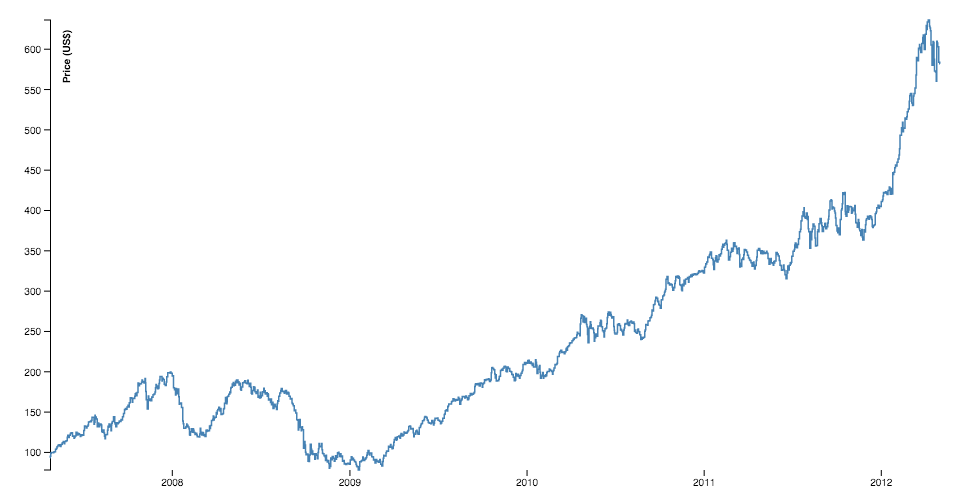 The line generator produces a spline or polyline, as in a line chart.
Lines also appear in many other visualization types, such as the links in hierarchical edge bundling.
# d3.line([x][, y]) · Source, Examples
Constructs a new line generator with the default settings.
If x or y are specified, sets the corresponding accessors to the specified function or number and returns this line generator.
# line(data) · Source, Examples
Generates a line for the given array of data.
Depending on this line generator’s associated curve, the given input data may need to be sorted by x-value before being passed to the line generator.
If the line generator has a context, then the line is rendered to this context as a sequence of path method calls and this function returns void.
Otherwise, a path data string is returned.
# line.x([x]) · Source, Examples
If x is specified, sets the x accessor to the specified function or number and returns this line generator.
If x is not specified, returns the current x accessor, which defaults to:
function x(d) {
return d[0];
}
When a line is generated, the x accessor will be invoked for each defined element in the input data array, being passed the element
The line generator produces a spline or polyline, as in a line chart.
Lines also appear in many other visualization types, such as the links in hierarchical edge bundling.
# d3.line([x][, y]) · Source, Examples
Constructs a new line generator with the default settings.
If x or y are specified, sets the corresponding accessors to the specified function or number and returns this line generator.
# line(data) · Source, Examples
Generates a line for the given array of data.
Depending on this line generator’s associated curve, the given input data may need to be sorted by x-value before being passed to the line generator.
If the line generator has a context, then the line is rendered to this context as a sequence of path method calls and this function returns void.
Otherwise, a path data string is returned.
# line.x([x]) · Source, Examples
If x is specified, sets the x accessor to the specified function or number and returns this line generator.
If x is not specified, returns the current x accessor, which defaults to:
function x(d) {
return d[0];
}
When a line is generated, the x accessor will be invoked for each defined element in the input data array, being passed the element d, the index i, and the array data as three arguments.
The default x accessor assumes that the input data are two-element arrays of numbers.
If your data are in a different format, or if you wish to transform the data before rendering, then you should specify a custom accessor.
For example, if x is a time scale and y is a linear scale:
var data = [
{date: new Date(2007, 3, 24), value: 93.24},
{date: new Date(2007, 3, 25), value: 95.35},
{date: new Date(2007, 3, 26), value: 98.84},
{date: new Date(2007, 3, 27), value: 99.92},
{date: new Date(2007, 3, 30), value: 99.80},
{date: new Date(2007, 4, 1), value: 99.47},
…
];
var line = d3.line()
.x(function(d) { return x(d.date); })
.y(function(d) { return y(d.value); });
# line.y([y]) · Source, Examples
If y is specified, sets the y accessor to the specified function or number and returns this line generator.
If y is not specified, returns the current y accessor, which defaults to:
function y(d) {
return d[1];
}
When a line is generated, the y accessor will be invoked for each defined element in the input data array, being passed the element d, the index i, and the array data as three arguments.
The default y accessor assumes that the input data are two-element arrays of numbers.
See line.x for more information.
# line.defined([defined]) · Source, Examples
If defined is specified, sets the defined accessor to the specified function or boolean and returns this line generator.
If defined is not specified, returns the current defined accessor, which defaults to:
function defined() {
return true;
}
The default accessor thus assumes that the input data is always defined.
When a line is generated, the defined accessor will be invoked for each element in the input data array, being passed the element d, the index i, and the array data as three arguments.
If the given element is defined (i.e., if the defined accessor returns a truthy value for this element), the x and y accessors will subsequently be evaluated and the point will be added to the current line segment.
Otherwise, the element will be skipped, the current line segment will be ended, and a new line segment will be generated for the next defined point.
As a result, the generated line may have several discrete segments.
For example:
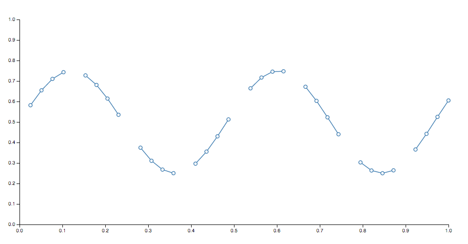 Note that if a line segment consists of only a single point, it may appear invisible unless rendered with rounded or square line caps.
In addition, some curves such as curveCardinalOpen only render a visible segment if it contains multiple points.
# line.curve([curve]) · Source, Examples
If curve is specified, sets the curve factory and returns this line generator.
If curve is not specified, returns the current curve factory, which defaults to curveLinear.
# line.context([context]) · Source, Examples
If context is specified, sets the context and returns this line generator.
If context is not specified, returns the current context, which defaults to null.
If the context is not null, then the generated line is rendered to this context as a sequence of path method calls.
Otherwise, a path data string representing the generated line is returned.
# d3.lineRadial() · Source, Examples
Note that if a line segment consists of only a single point, it may appear invisible unless rendered with rounded or square line caps.
In addition, some curves such as curveCardinalOpen only render a visible segment if it contains multiple points.
# line.curve([curve]) · Source, Examples
If curve is specified, sets the curve factory and returns this line generator.
If curve is not specified, returns the current curve factory, which defaults to curveLinear.
# line.context([context]) · Source, Examples
If context is specified, sets the context and returns this line generator.
If context is not specified, returns the current context, which defaults to null.
If the context is not null, then the generated line is rendered to this context as a sequence of path method calls.
Otherwise, a path data string representing the generated line is returned.
# d3.lineRadial() · Source, Examples
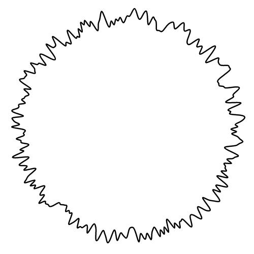 Constructs a new radial line generator with the default settings.
A radial line generator is equivalent to the standard Cartesian line generator, except the x and y accessors are replaced with angle and radius accessors.
Radial lines are always positioned relative to 0,0; use a transform (see: SVG, Canvas) to change the origin.
# lineRadial(data) · Source, Examples
Equivalent to line.
# lineRadial.angle([angle]) · Source, Examples
Equivalent to line.x, except the accessor returns the angle in radians, with 0 at -y (12 o’clock).
# lineRadial.radius([radius]) · Source, Examples
Equivalent to line.y, except the accessor returns the radius: the distance from the origin 0,0.
# lineRadial.defined([defined])
Equivalent to line.defined.
# lineRadial.curve([curve]) · Source, Examples
Equivalent to line.curve.
Note that curveMonotoneX or curveMonotoneY are not recommended for radial lines because they assume that the data is monotonic in x or y, which is typically untrue of radial lines.
# lineRadial.context([context])
Equivalent to line.context.
Constructs a new radial line generator with the default settings.
A radial line generator is equivalent to the standard Cartesian line generator, except the x and y accessors are replaced with angle and radius accessors.
Radial lines are always positioned relative to 0,0; use a transform (see: SVG, Canvas) to change the origin.
# lineRadial(data) · Source, Examples
Equivalent to line.
# lineRadial.angle([angle]) · Source, Examples
Equivalent to line.x, except the accessor returns the angle in radians, with 0 at -y (12 o’clock).
# lineRadial.radius([radius]) · Source, Examples
Equivalent to line.y, except the accessor returns the radius: the distance from the origin 0,0.
# lineRadial.defined([defined])
Equivalent to line.defined.
# lineRadial.curve([curve]) · Source, Examples
Equivalent to line.curve.
Note that curveMonotoneX or curveMonotoneY are not recommended for radial lines because they assume that the data is monotonic in x or y, which is typically untrue of radial lines.
# lineRadial.context([context])
Equivalent to line.context.
Areas
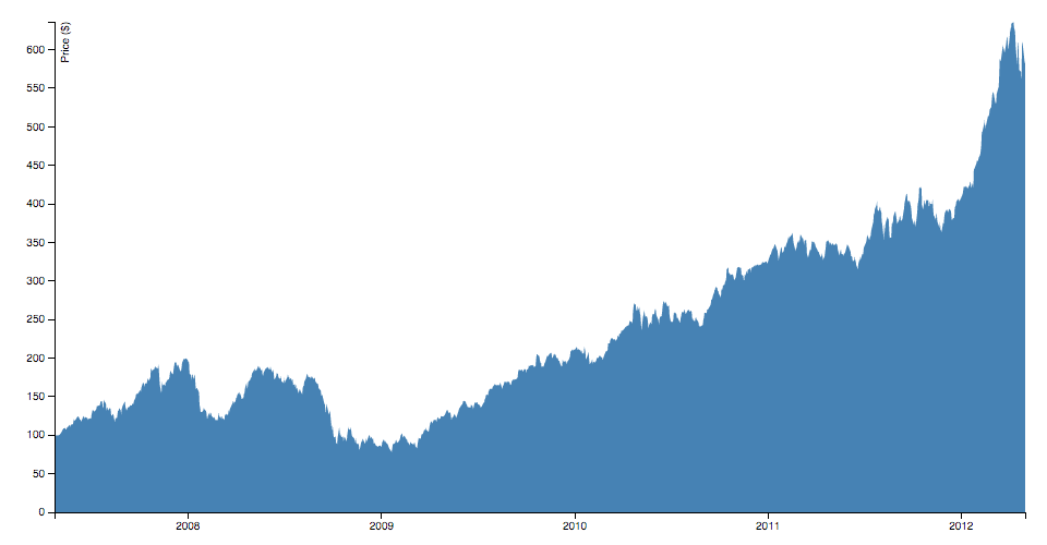
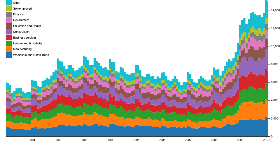
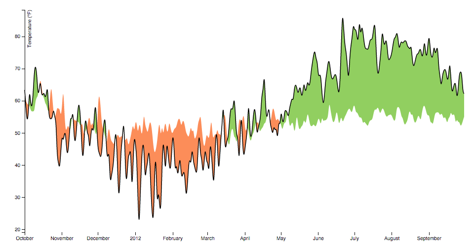 The area generator produces an area, as in an area chart.
An area is defined by two bounding lines, either splines or polylines.
Typically, the two lines share the same x-values (x0 = x1), differing only in y-value (y0 and y1); most commonly, y0 is defined as a constant representing zero.
The first line (the topline) is defined by x1 and y1 and is rendered first; the second line (the baseline) is defined by x0 and y0 and is rendered second, with the points in reverse order.
With a curveLinear curve, this produces a clockwise polygon.
# d3.area([x][, y0][, y1]) · Source
Constructs a new area generator with the default settings.
If x, y0 or y1 are specified, sets the corresponding accessors to the specified function or number and returns this area generator.
# area(data) · Source
Generates an area for the given array of data.
Depending on this area generator’s associated curve, the given input data may need to be sorted by x-value before being passed to the area generator.
If the area generator has a context, then the area is rendered to this context as a sequence of path method calls and this function returns void.
Otherwise, a path data string is returned.
# area.x([x]) · Source
If x is specified, sets x0 to x and x1 to null and returns this area generator.
If x is not specified, returns the current x0 accessor.
# area.x0([x]) · Source
If x is specified, sets the x0 accessor to the specified function or number and returns this area generator.
If x is not specified, returns the current x0 accessor, which defaults to:
function x(d) {
return d[0];
}
When an area is generated, the x0 accessor will be invoked for each defined element in the input data array, being passed the element
The area generator produces an area, as in an area chart.
An area is defined by two bounding lines, either splines or polylines.
Typically, the two lines share the same x-values (x0 = x1), differing only in y-value (y0 and y1); most commonly, y0 is defined as a constant representing zero.
The first line (the topline) is defined by x1 and y1 and is rendered first; the second line (the baseline) is defined by x0 and y0 and is rendered second, with the points in reverse order.
With a curveLinear curve, this produces a clockwise polygon.
# d3.area([x][, y0][, y1]) · Source
Constructs a new area generator with the default settings.
If x, y0 or y1 are specified, sets the corresponding accessors to the specified function or number and returns this area generator.
# area(data) · Source
Generates an area for the given array of data.
Depending on this area generator’s associated curve, the given input data may need to be sorted by x-value before being passed to the area generator.
If the area generator has a context, then the area is rendered to this context as a sequence of path method calls and this function returns void.
Otherwise, a path data string is returned.
# area.x([x]) · Source
If x is specified, sets x0 to x and x1 to null and returns this area generator.
If x is not specified, returns the current x0 accessor.
# area.x0([x]) · Source
If x is specified, sets the x0 accessor to the specified function or number and returns this area generator.
If x is not specified, returns the current x0 accessor, which defaults to:
function x(d) {
return d[0];
}
When an area is generated, the x0 accessor will be invoked for each defined element in the input data array, being passed the element d, the index i, and the array data as three arguments.
The default x0 accessor assumes that the input data are two-element arrays of numbers.
If your data are in a different format, or if you wish to transform the data before rendering, then you should specify a custom accessor.
For example, if x is a time scale and y is a linear scale:
var data = [
{date: new Date(2007, 3, 24), value: 93.24},
{date: new Date(2007, 3, 25), value: 95.35},
{date: new Date(2007, 3, 26), value: 98.84},
{date: new Date(2007, 3, 27), value: 99.92},
{date: new Date(2007, 3, 30), value: 99.80},
{date: new Date(2007, 4, 1), value: 99.47},
…
];
var area = d3.area()
.x(d => x(d.date))
.y1(d => y(d.value))
.y0(y(0));
# area.x1([x]) · Source
If x is specified, sets the x1 accessor to the specified function or number and returns this area generator.
If x is not specified, returns the current x1 accessor, which defaults to null, indicating that the previously-computed x0 value should be reused for the x1 value.
When an area is generated, the x1 accessor will be invoked for each defined element in the input data array, being passed the element d, the index i, and the array data as three arguments.
See area.x0 for more information.
# area.y([y]) · Source
If y is specified, sets y0 to y and y1 to null and returns this area generator.
If y is not specified, returns the current y0 accessor.
# area.y0([y]) · Source
If y is specified, sets the y0 accessor to the specified function or number and returns this area generator.
If y is not specified, returns the current y0 accessor, which defaults to:
function y() {
return 0;
}
When an area is generated, the y0 accessor will be invoked for each defined element in the input data array, being passed the element d, the index i, and the array data as three arguments.
See area.x0 for more information.
# area.y1([y]) · Source
If y is specified, sets the y1 accessor to the specified function or number and returns this area generator.
If y is not specified, returns the current y1 accessor, which defaults to:
function y(d) {
return d[1];
}
A null accessor is also allowed, indicating that the previously-computed y0 value should be reused for the y1 value.
When an area is generated, the y1 accessor will be invoked for each defined element in the input data array, being passed the element d, the index i, and the array data as three arguments.
See area.x0 for more information.
# area.defined([defined]) · Source
If defined is specified, sets the defined accessor to the specified function or boolean and returns this area generator.
If defined is not specified, returns the current defined accessor, which defaults to:
function defined() {
return true;
}
The default accessor thus assumes that the input data is always defined.
When an area is generated, the defined accessor will be invoked for each element in the input data array, being passed the element d, the index i, and the array data as three arguments.
If the given element is defined (i.e., if the defined accessor returns a truthy value for this element), the x0, x1, y0 and y1 accessors will subsequently be evaluated and the point will be added to the current area segment.
Otherwise, the element will be skipped, the current area segment will be ended, and a new area segment will be generated for the next defined point.
As a result, the generated area may have several discrete segments.
For example:
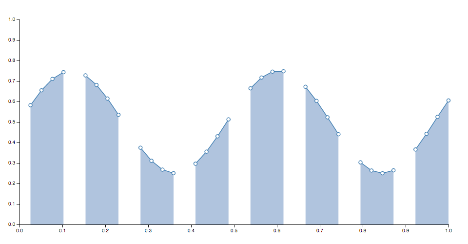 Note that if an area segment consists of only a single point, it may appear invisible unless rendered with rounded or square line caps.
In addition, some curves such as curveCardinalOpen only render a visible segment if it contains multiple points.
# area.curve([curve]) · Source
If curve is specified, sets the curve factory and returns this area generator.
If curve is not specified, returns the current curve factory, which defaults to curveLinear.
# area.context([context]) · Source
If context is specified, sets the context and returns this area generator.
If context is not specified, returns the current context, which defaults to null.
If the context is not null, then the generated area is rendered to this context as a sequence of path method calls.
Otherwise, a path data string representing the generated area is returned.
# area.lineX0() · Source
Note that if an area segment consists of only a single point, it may appear invisible unless rendered with rounded or square line caps.
In addition, some curves such as curveCardinalOpen only render a visible segment if it contains multiple points.
# area.curve([curve]) · Source
If curve is specified, sets the curve factory and returns this area generator.
If curve is not specified, returns the current curve factory, which defaults to curveLinear.
# area.context([context]) · Source
If context is specified, sets the context and returns this area generator.
If context is not specified, returns the current context, which defaults to null.
If the context is not null, then the generated area is rendered to this context as a sequence of path method calls.
Otherwise, a path data string representing the generated area is returned.
# area.lineX0() · Source
# area.lineY0() · Source
Returns a new line generator that has this area generator’s current defined accessor, curve and context.
The line’s x-accessor is this area’s x0-accessor, and the line’s y-accessor is this area’s y0-accessor.
# area.lineX1() · Source
Returns a new line generator that has this area generator’s current defined accessor, curve and context.
The line’s x-accessor is this area’s x1-accessor, and the line’s y-accessor is this area’s y0-accessor.
# area.lineY1() · Source
Returns a new line generator that has this area generator’s current defined accessor, curve and context.
The line’s x-accessor is this area’s x0-accessor, and the line’s y-accessor is this area’s y1-accessor.
# d3.areaRadial() · Source
 Constructs a new radial area generator with the default settings.
A radial area generator is equivalent to the standard Cartesian area generator, except the x and y accessors are replaced with angle and radius accessors.
Radial areas are always positioned relative to 0,0; use a transform (see: SVG, Canvas) to change the origin.
# areaRadial(data)
Equivalent to area.
# areaRadial.angle([angle]) · Source
Equivalent to area.x, except the accessor returns the angle in radians, with 0 at -y (12 o’clock).
# areaRadial.startAngle([angle]) · Source
Equivalent to area.x0, except the accessor returns the angle in radians, with 0 at -y (12 o’clock).
Note: typically angle is used instead of setting separate start and end angles.
# areaRadial.endAngle([angle]) · Source
Equivalent to area.x1, except the accessor returns the angle in radians, with 0 at -y (12 o’clock).
Note: typically angle is used instead of setting separate start and end angles.
# areaRadial.radius([radius]) · Source
Equivalent to area.y, except the accessor returns the radius: the distance from the origin 0,0.
# areaRadial.innerRadius([radius]) · Source
Equivalent to area.y0, except the accessor returns the radius: the distance from the origin 0,0.
# areaRadial.outerRadius([radius]) · Source
Equivalent to area.y1, except the accessor returns the radius: the distance from the origin 0,0.
# areaRadial.defined([defined])
Equivalent to area.defined.
# areaRadial.curve([curve]) · Source
Equivalent to area.curve.
Note that curveMonotoneX or curveMonotoneY are not recommended for radial areas because they assume that the data is monotonic in x or y, which is typically untrue of radial areas.
# areaRadial.context([context])
Equivalent to line.context.
# areaRadial.lineStartAngle() · Source
Constructs a new radial area generator with the default settings.
A radial area generator is equivalent to the standard Cartesian area generator, except the x and y accessors are replaced with angle and radius accessors.
Radial areas are always positioned relative to 0,0; use a transform (see: SVG, Canvas) to change the origin.
# areaRadial(data)
Equivalent to area.
# areaRadial.angle([angle]) · Source
Equivalent to area.x, except the accessor returns the angle in radians, with 0 at -y (12 o’clock).
# areaRadial.startAngle([angle]) · Source
Equivalent to area.x0, except the accessor returns the angle in radians, with 0 at -y (12 o’clock).
Note: typically angle is used instead of setting separate start and end angles.
# areaRadial.endAngle([angle]) · Source
Equivalent to area.x1, except the accessor returns the angle in radians, with 0 at -y (12 o’clock).
Note: typically angle is used instead of setting separate start and end angles.
# areaRadial.radius([radius]) · Source
Equivalent to area.y, except the accessor returns the radius: the distance from the origin 0,0.
# areaRadial.innerRadius([radius]) · Source
Equivalent to area.y0, except the accessor returns the radius: the distance from the origin 0,0.
# areaRadial.outerRadius([radius]) · Source
Equivalent to area.y1, except the accessor returns the radius: the distance from the origin 0,0.
# areaRadial.defined([defined])
Equivalent to area.defined.
# areaRadial.curve([curve]) · Source
Equivalent to area.curve.
Note that curveMonotoneX or curveMonotoneY are not recommended for radial areas because they assume that the data is monotonic in x or y, which is typically untrue of radial areas.
# areaRadial.context([context])
Equivalent to line.context.
# areaRadial.lineStartAngle() · Source
# areaRadial.lineInnerRadius() · Source
Returns a new radial line generator that has this radial area generator’s current defined accessor, curve and context.
The line’s angle accessor is this area’s start angle accessor, and the line’s radius accessor is this area’s inner radius accessor.
# areaRadial.lineEndAngle() · Source
Returns a new radial line generator that has this radial area generator’s current defined accessor, curve and context.
The line’s angle accessor is this area’s end angle accessor, and the line’s radius accessor is this area’s inner radius accessor.
# areaRadial.lineOuterRadius() · Source
Returns a new radial line generator that has this radial area generator’s current defined accessor, curve and context.
The line’s angle accessor is this area’s start angle accessor, and the line’s radius accessor is this area’s outer radius accessor.
Curves
While lines are defined as a sequence of two-dimensional [x, y] points, and areas are similarly defined by a topline and a baseline, there remains the task of transforming this discrete representation into a continuous shape: i.e., how to interpolate between the points.
A variety of curves are provided for this purpose.
Curves are typically not constructed or used directly, instead being passed to line.curve and area.curve.
For example:
var line = d3.line(d => d.date, d => d.value)
.curve(d3.curveCatmullRom.alpha(0.5));
# d3.curveBasis(context) · Source
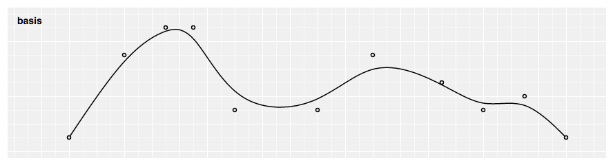 Produces a cubic basis spline using the specified control points.
The first and last points are triplicated such that the spline starts at the first point and ends at the last point, and is tangent to the line between the first and second points, and to the line between the penultimate and last points.
# d3.curveBasisClosed(context) · Source
Produces a cubic basis spline using the specified control points.
The first and last points are triplicated such that the spline starts at the first point and ends at the last point, and is tangent to the line between the first and second points, and to the line between the penultimate and last points.
# d3.curveBasisClosed(context) · Source
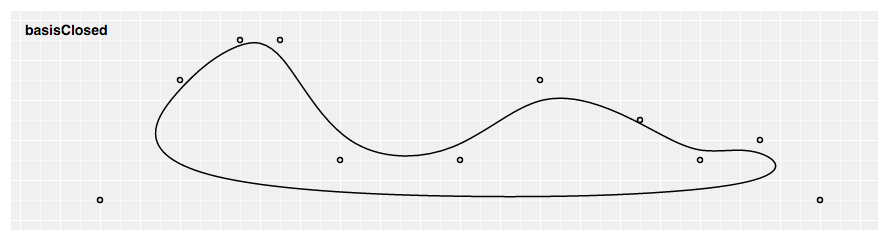 Produces a closed cubic basis spline using the specified control points.
When a line segment ends, the first three control points are repeated, producing a closed loop with C2 continuity.
# d3.curveBasisOpen(context) · Source
Produces a closed cubic basis spline using the specified control points.
When a line segment ends, the first three control points are repeated, producing a closed loop with C2 continuity.
# d3.curveBasisOpen(context) · Source
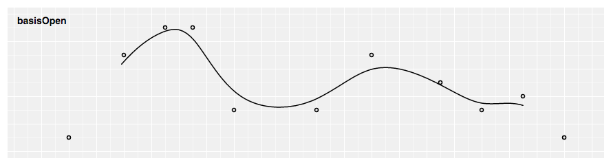 Produces a cubic basis spline using the specified control points.
Unlike basis, the first and last points are not repeated, and thus the curve typically does not intersect these points.
# d3.curveBundle(context) · Source
Produces a cubic basis spline using the specified control points.
Unlike basis, the first and last points are not repeated, and thus the curve typically does not intersect these points.
# d3.curveBundle(context) · Source
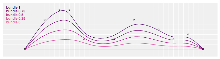 Produces a straightened cubic basis spline using the specified control points, with the spline straightened according to the curve’s beta, which defaults to 0.85.
This curve is typically used in hierarchical edge bundling to disambiguate connections, as proposed by Danny Holten in Hierarchical Edge Bundles: Visualization of Adjacency Relations in Hierarchical Data.
This curve does not implement curve.areaStart and curve.areaEnd; it is intended to work with d3.line, not d3.area.
# bundle.beta(beta) · Source
Returns a bundle curve with the specified beta in the range [0, 1], representing the bundle strength.
If beta equals zero, a straight line between the first and last point is produced; if beta equals one, a standard basis spline is produced.
For example:
var line = d3.line().curve(d3.curveBundle.beta(0.5));
# d3.curveCardinal(context) · Source
Produces a straightened cubic basis spline using the specified control points, with the spline straightened according to the curve’s beta, which defaults to 0.85.
This curve is typically used in hierarchical edge bundling to disambiguate connections, as proposed by Danny Holten in Hierarchical Edge Bundles: Visualization of Adjacency Relations in Hierarchical Data.
This curve does not implement curve.areaStart and curve.areaEnd; it is intended to work with d3.line, not d3.area.
# bundle.beta(beta) · Source
Returns a bundle curve with the specified beta in the range [0, 1], representing the bundle strength.
If beta equals zero, a straight line between the first and last point is produced; if beta equals one, a standard basis spline is produced.
For example:
var line = d3.line().curve(d3.curveBundle.beta(0.5));
# d3.curveCardinal(context) · Source
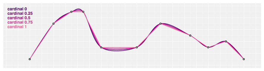 Produces a cubic cardinal spline using the specified control points, with one-sided differences used for the first and last piece.
The default tension is 0.
# d3.curveCardinalClosed(context) · Source
Produces a cubic cardinal spline using the specified control points, with one-sided differences used for the first and last piece.
The default tension is 0.
# d3.curveCardinalClosed(context) · Source
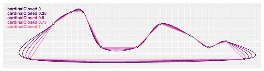 Produces a closed cubic cardinal spline using the specified control points.
When a line segment ends, the first three control points are repeated, producing a closed loop.
The default tension is 0.
# d3.curveCardinalOpen(context) · Source
Produces a closed cubic cardinal spline using the specified control points.
When a line segment ends, the first three control points are repeated, producing a closed loop.
The default tension is 0.
# d3.curveCardinalOpen(context) · Source
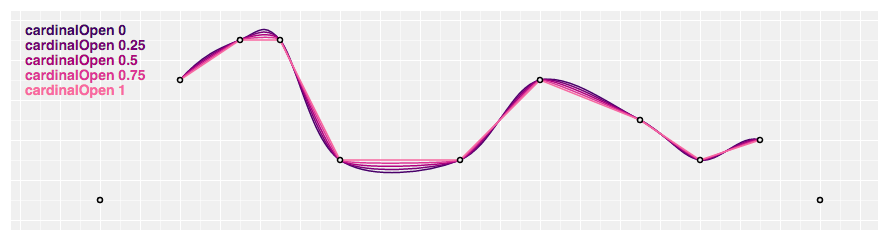 Produces a cubic cardinal spline using the specified control points.
Unlike curveCardinal, one-sided differences are not used for the first and last piece, and thus the curve starts at the second point and ends at the penultimate point.
The default tension is 0.
# cardinal.tension(tension) · Source
Returns a cardinal curve with the specified tension in the range [0, 1].
The tension determines the length of the tangents: a tension of one yields all zero tangents, equivalent to curveLinear; a tension of zero produces a uniform Catmull–Rom spline.
For example:
var line = d3.line().curve(d3.curveCardinal.tension(0.5));
# d3.curveCatmullRom(context) · Source
Produces a cubic cardinal spline using the specified control points.
Unlike curveCardinal, one-sided differences are not used for the first and last piece, and thus the curve starts at the second point and ends at the penultimate point.
The default tension is 0.
# cardinal.tension(tension) · Source
Returns a cardinal curve with the specified tension in the range [0, 1].
The tension determines the length of the tangents: a tension of one yields all zero tangents, equivalent to curveLinear; a tension of zero produces a uniform Catmull–Rom spline.
For example:
var line = d3.line().curve(d3.curveCardinal.tension(0.5));
# d3.curveCatmullRom(context) · Source
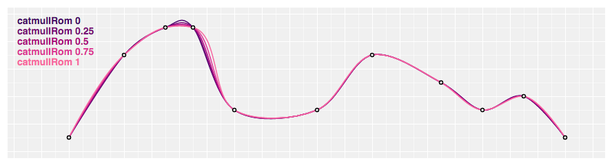 Produces a cubic Catmull–Rom spline using the specified control points and the parameter alpha, which defaults to 0.5, as proposed by Yuksel et al.
in On the Parameterization of Catmull–Rom Curves, with one-sided differences used for the first and last piece.
# d3.curveCatmullRomClosed(context) · Source
Produces a cubic Catmull–Rom spline using the specified control points and the parameter alpha, which defaults to 0.5, as proposed by Yuksel et al.
in On the Parameterization of Catmull–Rom Curves, with one-sided differences used for the first and last piece.
# d3.curveCatmullRomClosed(context) · Source
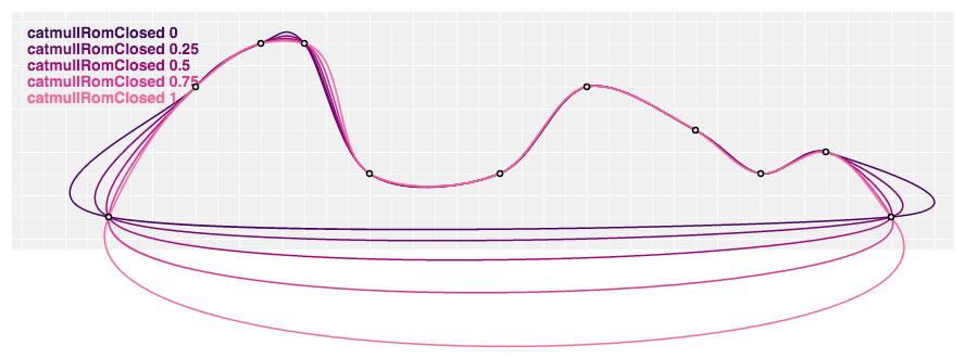 Produces a closed cubic Catmull–Rom spline using the specified control points and the parameter alpha, which defaults to 0.5, as proposed by Yuksel et al.
When a line segment ends, the first three control points are repeated, producing a closed loop.
# d3.curveCatmullRomOpen(context) · Source
Produces a closed cubic Catmull–Rom spline using the specified control points and the parameter alpha, which defaults to 0.5, as proposed by Yuksel et al.
When a line segment ends, the first three control points are repeated, producing a closed loop.
# d3.curveCatmullRomOpen(context) · Source
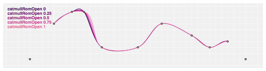 Produces a cubic Catmull–Rom spline using the specified control points and the parameter alpha, which defaults to 0.5, as proposed by Yuksel et al.
Unlike curveCatmullRom, one-sided differences are not used for the first and last piece, and thus the curve starts at the second point and ends at the penultimate point.
# catmullRom.alpha(alpha) · Source
Returns a cubic Catmull–Rom curve with the specified alpha in the range [0, 1].
If alpha is zero, produces a uniform spline, equivalent to curveCardinal with a tension of zero; if alpha is one, produces a chordal spline; if alpha is 0.5, produces a centripetal spline.
Centripetal splines are recommended to avoid self-intersections and overshoot.
For example:
var line = d3.line().curve(d3.curveCatmullRom.alpha(0.5));
# d3.curveLinear(context) · Source
Produces a cubic Catmull–Rom spline using the specified control points and the parameter alpha, which defaults to 0.5, as proposed by Yuksel et al.
Unlike curveCatmullRom, one-sided differences are not used for the first and last piece, and thus the curve starts at the second point and ends at the penultimate point.
# catmullRom.alpha(alpha) · Source
Returns a cubic Catmull–Rom curve with the specified alpha in the range [0, 1].
If alpha is zero, produces a uniform spline, equivalent to curveCardinal with a tension of zero; if alpha is one, produces a chordal spline; if alpha is 0.5, produces a centripetal spline.
Centripetal splines are recommended to avoid self-intersections and overshoot.
For example:
var line = d3.line().curve(d3.curveCatmullRom.alpha(0.5));
# d3.curveLinear(context) · Source
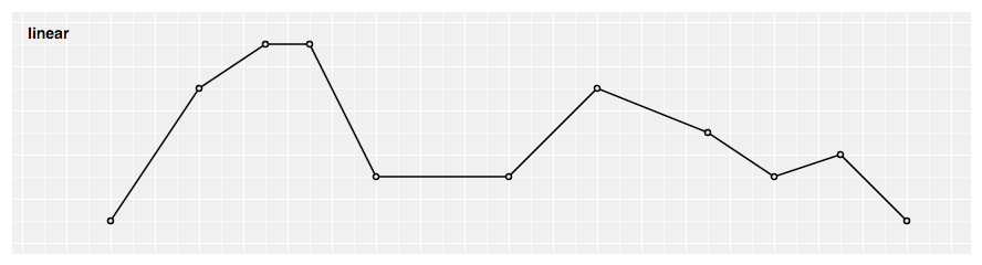 Produces a polyline through the specified points.
# d3.curveLinearClosed(context) · Source
Produces a polyline through the specified points.
# d3.curveLinearClosed(context) · Source
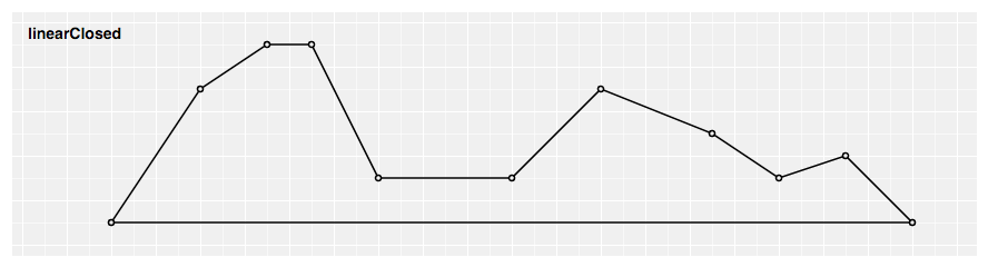 Produces a closed polyline through the specified points by repeating the first point when the line segment ends.
# d3.curveMonotoneX(context) · Source
Produces a closed polyline through the specified points by repeating the first point when the line segment ends.
# d3.curveMonotoneX(context) · Source
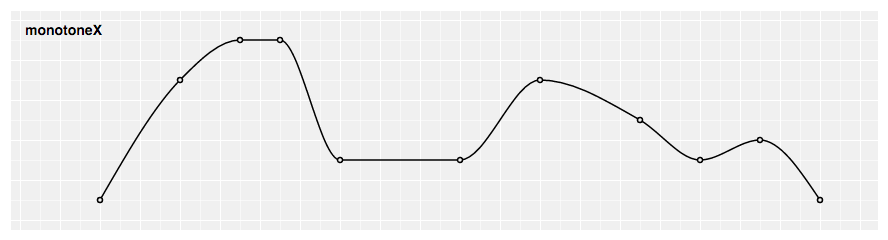 Produces a cubic spline that preserves monotonicity in y, assuming monotonicity in x, as proposed by Steffen in A simple method for monotonic interpolation in one dimension: “a smooth curve with continuous first-order derivatives that passes through any given set of data points without spurious oscillations.
Local extrema can occur only at grid points where they are given by the data, but not in between two adjacent grid points.”
# d3.curveMonotoneY(context) · Source
Produces a cubic spline that preserves monotonicity in y, assuming monotonicity in x, as proposed by Steffen in A simple method for monotonic interpolation in one dimension: “a smooth curve with continuous first-order derivatives that passes through any given set of data points without spurious oscillations.
Local extrema can occur only at grid points where they are given by the data, but not in between two adjacent grid points.”
# d3.curveMonotoneY(context) · Source
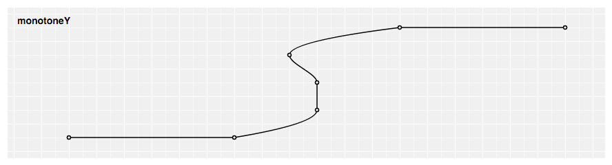 Produces a cubic spline that preserves monotonicity in x, assuming monotonicity in y, as proposed by Steffen in A simple method for monotonic interpolation in one dimension: “a smooth curve with continuous first-order derivatives that passes through any given set of data points without spurious oscillations.
Local extrema can occur only at grid points where they are given by the data, but not in between two adjacent grid points.”
# d3.curveNatural(context) · Source
Produces a cubic spline that preserves monotonicity in x, assuming monotonicity in y, as proposed by Steffen in A simple method for monotonic interpolation in one dimension: “a smooth curve with continuous first-order derivatives that passes through any given set of data points without spurious oscillations.
Local extrema can occur only at grid points where they are given by the data, but not in between two adjacent grid points.”
# d3.curveNatural(context) · Source
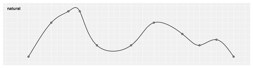 Produces a natural cubic spline with the second derivative of the spline set to zero at the endpoints.
# d3.curveStep(context) · Source
Produces a natural cubic spline with the second derivative of the spline set to zero at the endpoints.
# d3.curveStep(context) · Source
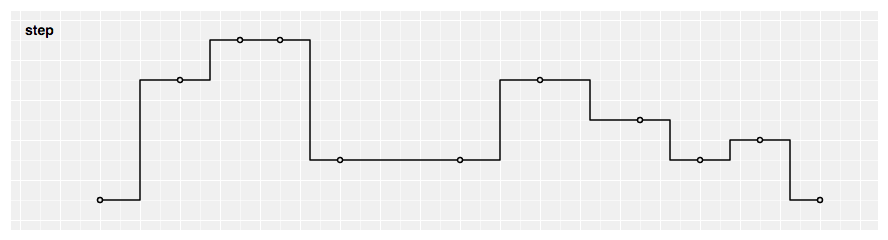 Produces a piecewise constant function (a step function) consisting of alternating horizontal and vertical lines.
The y-value changes at the midpoint of each pair of adjacent x-values.
# d3.curveStepAfter(context) · Source
Produces a piecewise constant function (a step function) consisting of alternating horizontal and vertical lines.
The y-value changes at the midpoint of each pair of adjacent x-values.
# d3.curveStepAfter(context) · Source
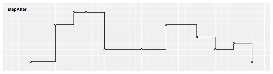 Produces a piecewise constant function (a step function) consisting of alternating horizontal and vertical lines.
The y-value changes after the x-value.
# d3.curveStepBefore(context) · Source
Produces a piecewise constant function (a step function) consisting of alternating horizontal and vertical lines.
The y-value changes after the x-value.
# d3.curveStepBefore(context) · Source
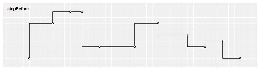 Produces a piecewise constant function (a step function) consisting of alternating horizontal and vertical lines.
The y-value changes before the x-value.
Produces a piecewise constant function (a step function) consisting of alternating horizontal and vertical lines.
The y-value changes before the x-value.
Custom Curves
Curves are typically not used directly, instead being passed to line.curve and area.curve.
However, you can define your own curve implementation should none of the built-in curves satisfy your needs using the following interface.
You can also use this low-level interface with a built-in curve type as an alternative to the line and area generators.
# curve.areaStart() · Source
Indicates the start of a new area segment.
Each area segment consists of exactly two line segments: the topline, followed by the baseline, with the baseline points in reverse order.
# curve.areaEnd() · Source
Indicates the end of the current area segment.
# curve.lineStart() · Source
Indicates the start of a new line segment.
Zero or more points will follow.
# curve.lineEnd() · Source
Indicates the end of the current line segment.
# curve.point(x, y) · Source
Indicates a new point in the current line segment with the given x- and y-values.
Links
The link shape generates a smooth cubic Bézier curve from a source point to a target point.
The tangents of the curve at the start and end are either vertical, horizontal or radial.
# d3.linkVertical() · Source
Returns a new link generator with vertical tangents.
For example, to visualize links in a tree diagram rooted on the top edge of the display, you might say:
var link = d3.linkVertical()
.x(function(d) { return d.x; })
.y(function(d) { return d.y; });
# d3.linkHorizontal() · Source
Returns a new link generator with horizontal tangents.
For example, to visualize links in a tree diagram rooted on the left edge of the display, you might say:
var link = d3.linkHorizontal()
.x(function(d) { return d.y; })
.y(function(d) { return d.x; });
# link(arguments…) · Source
Generates a link for the given arguments.
The arguments are arbitrary; they are simply propagated to the link generator’s accessor functions along with the this object.
For example, with the default settings, an object expected:
link({
source: [100, 100],
target: [300, 300]
});
# link.source([source]) · Source
If source is specified, sets the source accessor to the specified function and returns this link generator.
If source is not specified, returns the current source accessor, which defaults to:
function source(d) {
return d.source;
}
# link.target([target]) · Source
If target is specified, sets the target accessor to the specified function and returns this link generator.
If target is not specified, returns the current target accessor, which defaults to:
function target(d) {
return d.target;
}
# link.x([x]) · Source
If x is specified, sets the x-accessor to the specified function or number and returns this link generator.
If x is not specified, returns the current x-accessor, which defaults to:
function x(d) {
return d[0];
}
# link.y([y]) · Source
If y is specified, sets the y-accessor to the specified function or number and returns this link generator.
If y is not specified, returns the current y-accessor, which defaults to:
function y(d) {
return d[1];
}
# link.context([context]) · Source
If context is specified, sets the context and returns this link generator.
If context is not specified, returns the current context, which defaults to null.
If the context is not null, then the generated link is rendered to this context as a sequence of path method calls.
Otherwise, a path data string representing the generated link is returned.
See also d3-path.
# d3.linkRadial() · Source
Returns a new link generator with radial tangents.
For example, to visualize links in a tree diagram rooted in the center of the display, you might say:
var link = d3.linkRadial()
.angle(function(d) { return d.x; })
.radius(function(d) { return d.y; });
# linkRadial.angle([angle]) · Source
Equivalent to link.x, except the accessor returns the angle in radians, with 0 at -y (12 o’clock).
# linkRadial.radius([radius]) · Source
Equivalent to link.y, except the accessor returns the radius: the distance from the origin 0,0.
Symbols

 Symbols provide a categorical shape encoding as is commonly used in scatterplots.
Symbols are always centered at 0,0; use a transform (see: SVG, Canvas) to move the symbol to a different position.
# d3.symbol([type][, size]) · Source, Examples
Constructs a new symbol generator of the specified type and size.
If not specified, type defaults to a circle, and size defaults to 64.
# symbol(arguments…) · Source, Examples
Generates a symbol for the given arguments.
The arguments are arbitrary; they are simply propagated to the symbol generator’s accessor functions along with the
Symbols provide a categorical shape encoding as is commonly used in scatterplots.
Symbols are always centered at 0,0; use a transform (see: SVG, Canvas) to move the symbol to a different position.
# d3.symbol([type][, size]) · Source, Examples
Constructs a new symbol generator of the specified type and size.
If not specified, type defaults to a circle, and size defaults to 64.
# symbol(arguments…) · Source, Examples
Generates a symbol for the given arguments.
The arguments are arbitrary; they are simply propagated to the symbol generator’s accessor functions along with the this object.
For example, with the default settings, no arguments are needed to produce a circle with area 64 square pixels.
If the symbol generator has a context, then the symbol is rendered to this context as a sequence of path method calls and this function returns void.
Otherwise, a path data string is returned.
# symbol.type([type]) · Source, Examples
If type is specified, sets the symbol type to the specified function or symbol type and returns this symbol generator.
If type is a function, the symbol generator’s arguments and this are passed through.
(See selection.attr if you are using d3-selection.) If type is not specified, returns the current symbol type accessor, which defaults to:
function type() {
return circle;
}
See symbols for the set of built-in symbol types.
To implement a custom symbol type, pass an object that implements symbolType.draw.
# symbol.size([size]) · Source, Examples
If size is specified, sets the size to the specified function or number and returns this symbol generator.
If size is a function, the symbol generator’s arguments and this are passed through.
(See selection.attr if you are using d3-selection.) If size is not specified, returns the current size accessor, which defaults to:
function size() {
return 64;
}
Specifying the size as a function is useful for constructing a scatterplot with a size encoding.
If you wish to scale the symbol to fit a given bounding box, rather than by area, try SVG’s getBBox.
# symbol.context([context]) · Source
If context is specified, sets the context and returns this symbol generator.
If context is not specified, returns the current context, which defaults to null.
If the context is not null, then the generated symbol is rendered to this context as a sequence of path method calls.
Otherwise, a path data string representing the generated symbol is returned.
# d3.symbols · Source, Examples
An array containing the set of all built-in symbol types: circle, cross, diamond, square, star, triangle, and wye.
Useful for constructing the range of an ordinal scale should you wish to use a shape encoding for categorical data.
# d3.symbolCircle · Source, Examples
The circle symbol type.
# d3.symbolCross · Source, Examples
The Greek cross symbol type, with arms of equal length.
# d3.symbolDiamond · Source, Examples
The rhombus symbol type.
# d3.symbolSquare · Source, Examples
The square symbol type.
# d3.symbolStar · Source, Examples
The pentagonal star (pentagram) symbol type.
# d3.symbolTriangle · Source, Examples
The up-pointing triangle symbol type.
# d3.symbolWye · Source, Examples
The Y-shape symbol type.
# d3.pointRadial(angle, radius) · Source, Examples
Returns the point [x, y] for the given angle in radians, with 0 at -y (12 o’clock) and positive angles proceeding clockwise, and the given radius.
Custom Symbol Types
Symbol types are typically not used directly, instead being passed to symbol.type.
However, you can define your own symbol type implementation should none of the built-in types satisfy your needs using the following interface.
You can also use this low-level interface with a built-in symbol type as an alternative to the symbol generator.
# symbolType.draw(context, size)
Renders this symbol type to the specified context with the specified size in square pixels.
The context implements the CanvasPathMethods interface.
(Note that this is a subset of the CanvasRenderingContext2D interface!)
Stacks
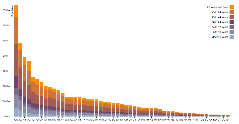
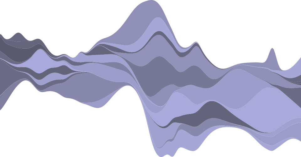 Some shape types can be stacked, placing one shape adjacent to another.
For example, a bar chart of monthly sales might be broken down into a multi-series bar chart by product category, stacking bars vertically.
This is equivalent to subdividing a bar chart by an ordinal dimension (such as product category) and applying a color encoding.
Stacked charts can show overall value and per-category value simultaneously; however, it is typically harder to compare across categories, as only the bottom layer of the stack is aligned.
So, chose the stack order carefully, and consider a streamgraph.
(See also grouped charts.)
Like the pie generator, the stack generator does not produce a shape directly.
Instead it computes positions which you can then pass to an area generator or use directly, say to position bars.
# d3.stack() · Source
Constructs a new stack generator with the default settings.
# stack(data[, arguments…]) · Source
Generates a stack for the given array of data, returning an array representing each series.
Any additional arguments are arbitrary; they are simply propagated to accessors along with the
Some shape types can be stacked, placing one shape adjacent to another.
For example, a bar chart of monthly sales might be broken down into a multi-series bar chart by product category, stacking bars vertically.
This is equivalent to subdividing a bar chart by an ordinal dimension (such as product category) and applying a color encoding.
Stacked charts can show overall value and per-category value simultaneously; however, it is typically harder to compare across categories, as only the bottom layer of the stack is aligned.
So, chose the stack order carefully, and consider a streamgraph.
(See also grouped charts.)
Like the pie generator, the stack generator does not produce a shape directly.
Instead it computes positions which you can then pass to an area generator or use directly, say to position bars.
# d3.stack() · Source
Constructs a new stack generator with the default settings.
# stack(data[, arguments…]) · Source
Generates a stack for the given array of data, returning an array representing each series.
Any additional arguments are arbitrary; they are simply propagated to accessors along with the this object.
The series are determined by the keys accessor; each series i in the returned array corresponds to the ith key.
Each series is an array of points, where each point j corresponds to the jth element in the input data.
Lastly, each point is represented as an array [y0, y1] where y0 is the lower value (baseline) and y1 is the upper value (topline); the difference between y0 and y1 corresponds to the computed value for this point.
The key for each series is available as series.key, and the index as series.index.
The input data element for each point is available as point.data.
For example, consider the following table representing monthly sales of fruits:
| Month |
Apples |
Bananas |
Cherries |
Dates |
| 1/2015 |
3840 |
1920 |
960 |
400 |
| 2/2015 |
1600 |
1440 |
960 |
400 |
| 3/2015 |
640 |
960 |
640 |
400 |
| 4/2015 |
320 |
480 |
640 |
400 |
This might be represented in JavaScript as an array of objects:
var data = [
{month: new Date(2015, 0, 1), apples: 3840, bananas: 1920, cherries: 960, dates: 400},
{month: new Date(2015, 1, 1), apples: 1600, bananas: 1440, cherries: 960, dates: 400},
{month: new Date(2015, 2, 1), apples: 640, bananas: 960, cherries: 640, dates: 400},
{month: new Date(2015, 3, 1), apples: 320, bananas: 480, cherries: 640, dates: 400}
];
To produce a stack for this data:
var stack = d3.stack()
.keys(["apples", "bananas", "cherries", "dates"])
.order(d3.stackOrderNone)
.offset(d3.stackOffsetNone);
var series = stack(data);
The resulting array has one element per series.
Each series has one point per month, and each point has a lower and upper value defining the baseline and topline:
[
[[ 0, 3840], [ 0, 1600], [ 0, 640], [ 0, 320]], // apples
[[3840, 5760], [1600, 3040], [ 640, 1600], [ 320, 800]], // bananas
[[5760, 6720], [3040, 4000], [1600, 2240], [ 800, 1440]], // cherries
[[6720, 7120], [4000, 4400], [2240, 2640], [1440, 1840]], // dates
]
Each series in then typically passed to an area generator to render an area chart, or used to construct rectangles for a bar chart.
# stack.keys([keys]) · Source
If keys is specified, sets the keys accessor to the specified function or array and returns this stack generator.
If keys is not specified, returns the current keys accessor, which defaults to the empty array.
A series (layer) is generated for each key.
Keys are typically strings, but they may be arbitrary values.
The series’ key is passed to the value accessor, along with each data point, to compute the point’s value.
# stack.value([value]) · Source
If value is specified, sets the value accessor to the specified function or number and returns this stack generator.
If value is not specified, returns the current value accessor, which defaults to:
function value(d, key) {
return d[key];
}
Thus, by default the stack generator assumes that the input data is an array of objects, with each object exposing named properties with numeric values; see stack for an example.
# stack.order([order]) · Source
If order is specified, sets the order accessor to the specified function or array and returns this stack generator.
If order is not specified, returns the current order accessor, which defaults to stackOrderNone; this uses the order given by the key accessor.
See stack orders for the built-in orders.
If order is a function, it is passed the generated series array and must return an array of numeric indexes representing the stack order.
For example, the default order is defined as:
function orderNone(series) {
var n = series.length, o = new Array(n);
while (--n >= 0) o[n] = n;
return o;
}
The stack order is computed prior to the offset; thus, the lower value for all points is zero at the time the order is computed.
The index attribute for each series is also not set until after the order is computed.
# stack.offset([offset]) · Source
If offset is specified, sets the offset accessor to the specified function and returns this stack generator.
If offset is not specified, returns the current offset acccesor, which defaults to stackOffsetNone; this uses a zero baseline.
See stack offsets for the built-in offsets.
The offset function is passed the generated series array and the order index array; it is then responsible for updating the lower and upper values in the series array.
For example, the default offset is defined as:
function offsetNone(series, order) {
if (!((n = series.length) > 1)) return;
for (var i = 1, s0, s1 = series[order[0]], n, m = s1.length; i < n; ++i) {
s0 = s1, s1 = series[order[i]];
for (var j = 0; j < m; ++j) {
s1[j][1] += s1[j][0] = s0[j][1];
}
}
}
Stack Orders
Stack orders are typically not used directly, but are instead passed to stack.order.
# d3.stackOrderAppearance(series) · Source
Returns a series order such that the earliest series (according to the maximum value) is at the bottom.
# d3.stackOrderAscending(series) · Source
Returns a series order such that the smallest series (according to the sum of values) is at the bottom.
# d3.stackOrderDescending(series) · Source
Returns a series order such that the largest series (according to the sum of values) is at the bottom.
# d3.stackOrderInsideOut(series) · Source
Returns a series order such that the earliest series (according to the maximum value) are on the inside and the later series are on the outside.
This order is recommended for streamgraphs in conjunction with the wiggle offset.
See Stacked Graphs—Geometry & Aesthetics by Byron & Wattenberg for more information.
# d3.stackOrderNone(series) · Source
Returns the given series order [0, 1, … n - 1] where n is the number of elements in series.
Thus, the stack order is given by the key accessor.
# d3.stackOrderReverse(series) · Source
Returns the reverse of the given series order [n - 1, n - 2, … 0] where n is the number of elements in series.
Thus, the stack order is given by the reverse of the key accessor.
Stack Offsets
Stack offsets are typically not used directly, but are instead passed to stack.offset.
# d3.stackOffsetExpand(series, order) · Source
Applies a zero baseline and normalizes the values for each point such that the topline is always one.
# d3.stackOffsetDiverging(series, order) · Source
Positive values are stacked above zero, negative values are stacked below zero, and zero values are stacked at zero.
# d3.stackOffsetNone(series, order) · Source
Applies a zero baseline.
# d3.stackOffsetSilhouette(series, order) · Source
Shifts the baseline down such that the center of the streamgraph is always at zero.
# d3.stackOffsetWiggle(series, order) · Source
Shifts the baseline so as to minimize the weighted wiggle of layers.
This offset is recommended for streamgraphs in conjunction with the inside-out order.
See Stacked Graphs—Geometry & Aesthetics by Bryon & Wattenberg for more information.
d3-time-format
This module provides a JavaScript implementation of the venerable strptime and strftime functions from the C standard library, and can be used to parse or format dates in a variety of locale-specific representations.
To format a date, create a formatter from a specifier (a string with the desired format directives, indicated by %); then pass a date to the formatter, which returns a string.
For example, to convert the current date to a human-readable string:
var formatTime = d3.timeFormat("%B %d, %Y");
formatTime(new Date); // "June 30, 2015"
Likewise, to convert a string back to a date, create a parser:
var parseTime = d3.timeParse("%B %d, %Y");
parseTime("June 30, 2015"); // Tue Jun 30 2015 00:00:00 GMT-0700 (PDT)
You can implement more elaborate conditional time formats, too.
For example, here’s a multi-scale time format using time intervals:
var formatMillisecond = d3.timeFormat(".%L"),
formatSecond = d3.timeFormat(":%S"),
formatMinute = d3.timeFormat("%I:%M"),
formatHour = d3.timeFormat("%I %p"),
formatDay = d3.timeFormat("%a %d"),
formatWeek = d3.timeFormat("%b %d"),
formatMonth = d3.timeFormat("%B"),
formatYear = d3.timeFormat("%Y");
function multiFormat(date) {
return (d3.timeSecond(date) < date ? formatMillisecond
: d3.timeMinute(date) < date ? formatSecond
: d3.timeHour(date) < date ? formatMinute
: d3.timeDay(date) < date ? formatHour
: d3.timeMonth(date) < date ? (d3.timeWeek(date) < date ? formatDay : formatWeek)
: d3.timeYear(date) < date ? formatMonth
: formatYear)(date);
}
This module is used by D3 time scales to generate human-readable ticks.
Installing
If you use NPM, npm install d3-time-format.
Otherwise, download the latest release.
You can also load directly from d3js.org, either as a standalone library or as part of D3.
AMD, CommonJS, and vanilla environments are supported.
In vanilla, a d3 global is exported:
<script src="https://d3js.org/d3-time.v2.min.js"></script>
<script src="https://d3js.org/d3-time-format.v3.min.js"></script>
<script>
var format = d3.timeFormat("%x");
</script>
Locale files are published to npm and can be loaded using d3.json.
For example, to set Russian as the default locale:
d3.json("https://cdn.jsdelivr.net/npm/d3-time-format@3/locale/ru-RU.json", function(error, locale) {
if (error) throw error;
d3.timeFormatDefaultLocale(locale);
var format = d3.timeFormat("%c");
console.log(format(new Date)); // , 5 2016 .
10:31:59
});
API Reference
# d3.timeFormat(specifier) · Source
An alias for locale.format on the default locale.
# d3.timeParse(specifier) · Source
An alias for locale.parse on the default locale.
# d3.utcFormat(specifier) · Source
An alias for locale.utcFormat on the default locale.
# d3.utcParse(specifier) · Source
An alias for locale.utcParse on the default locale.
# d3.isoFormat · Source
The full ISO 8601 UTC time formatter.
Where available, this method will use Date.toISOString to format.
# d3.isoParse · Source
The full ISO 8601 UTC time parser.
Where available, this method will use the Date constructor to parse strings.
If you depend on strict validation of the input format according to ISO 8601, you should construct a UTC parser function:
var strictIsoParse = d3.utcParse("%Y-%m-%dT%H:%M:%S.%LZ");
# locale.format(specifier) · Source
Returns a new formatter for the given string specifier.
The specifier string may contain the following directives:
%a - abbreviated weekday name.*
%A - full weekday name.*
%b - abbreviated month name.*
%B - full month name.*
%c - the locale’s date and time, such as %x, %X.*
%d - zero-padded day of the month as a decimal number [01,31].
%e - space-padded day of the month as a decimal number [ 1,31]; equivalent to %_d.
%f - microseconds as a decimal number [000000, 999999].
%g - ISO 8601 week-based year without century as a decimal number [00,99].
%G - ISO 8601 week-based year with century as a decimal number.
%H - hour (24-hour clock) as a decimal number [00,23].
%I - hour (12-hour clock) as a decimal number [01,12].
%j - day of the year as a decimal number [001,366].
%m - month as a decimal number [01,12].
%M - minute as a decimal number [00,59].
%L - milliseconds as a decimal number [000, 999].
%p - either AM or PM.*
%q - quarter of the year as a decimal number [1,4].
%Q - milliseconds since UNIX epoch.
%s - seconds since UNIX epoch.
%S - second as a decimal number [00,61].
%u - Monday-based (ISO 8601) weekday as a decimal number [1,7].
%U - Sunday-based week of the year as a decimal number [00,53].
%V - ISO 8601 week of the year as a decimal number [01, 53].
%w - Sunday-based weekday as a decimal number [0,6].
%W - Monday-based week of the year as a decimal number [00,53].
%x - the locale’s date, such as %-m/%-d/%Y.*
%X - the locale’s time, such as %-I:%M:%S %p.*
%y - year without century as a decimal number [00,99].
%Y - year with century as a decimal number, such as 1999.
%Z - time zone offset, such as -0700, -07:00, -07, or Z.
%% - a literal percent sign (%).
Directives marked with an asterisk (*) may be affected by the locale definition.
For %U, all days in a new year preceding the first Sunday are considered to be in week 0.
For %W, all days in a new year preceding the first Monday are considered to be in week 0.
Week numbers are computed using interval.count.
For example, 2015-52 and 2016-00 represent Monday, December 28, 2015, while 2015-53 and 2016-01 represent Monday, January 4, 2016.
This differs from the ISO week date specification (%V), which uses a more complicated definition!
For %V,%g and %G, per the strftime man page:
In this system, weeks start on a Monday, and are numbered from 01, for the first week, up to 52 or 53, for the last week.
Week 1 is the first week where four or more days fall within the new year (or, synonymously, week 01 is: the first week of the year that contains a Thursday; or, the week that has 4 January in it).
If the ISO week number belongs to the previous or next year, that year is used instead.
The % sign indicating a directive may be immediately followed by a padding modifier:
0 - zero-padding
_ - space-padding
- - disable padding
If no padding modifier is specified, the default is 0 for all directives except %e, which defaults to _.
(In some implementations of strftime and strptime, a directive may include an optional field width or precision; this feature is not yet implemented.)
The returned function formats a specified date, returning the corresponding string.
var formatMonth = d3.timeFormat("%B"),
formatDay = d3.timeFormat("%A"),
date = new Date(2014, 4, 1); // Thu May 01 2014 00:00:00 GMT-0700 (PDT)
formatMonth(date); // "May"
formatDay(date); // "Thursday"
# locale.parse(specifier) · Source
Returns a new parser for the given string specifier.
The specifier string may contain the same directives as locale.format.
The %d and %e directives are considered equivalent for parsing.
The returned function parses a specified string, returning the corresponding date or null if the string could not be parsed according to this format’s specifier.
Parsing is strict: if the specified string does not exactly match the associated specifier, this method returns null.
For example, if the associated specifier is %Y-%m-%dT%H:%M:%SZ, then the string "2011-07-01T19:15:28Z" will be parsed as expected, but "2011-07-01T19:15:28", "2011-07-01 19:15:28" and "2011-07-01" will return null.
(Note that the literal Z here is different from the time zone offset directive %Z.) If a more flexible parser is desired, try multiple formats sequentially until one returns non-null.
# locale.utcFormat(specifier) · Source
Equivalent to locale.format, except all directives are interpreted as Coordinated Universal Time (UTC) rather than local time.
# locale.utcParse(specifier) · Source
Equivalent to locale.parse, except all directives are interpreted as Coordinated Universal Time (UTC) rather than local time.
Locales
# d3.timeFormatLocale(definition) · Source
Returns a locale object for the specified definition with locale.format, locale.parse, locale.utcFormat, locale.utcParse methods.
The definition must include the following properties:
dateTime - the date and time (%c) format specifier (e.g., "%a %b %e %X %Y").
date - the date (%x) format specifier (e.g., "%m/%d/%Y").
time - the time (%X) format specifier (e.g., "%H:%M:%S").
periods - the A.M.
and P.M.
equivalents (e.g., ["AM", "PM"]).
days - the full names of the weekdays, starting with Sunday.
shortDays - the abbreviated names of the weekdays, starting with Sunday.
months - the full names of the months (starting with January).
shortMonths - the abbreviated names of the months (starting with January).
For an example, see Localized Time Axis II.
# d3.timeFormatDefaultLocale(definition) · Source
Equivalent to d3.timeFormatLocale, except it also redefines d3.timeFormat, d3.timeParse, d3.utcFormat and d3.utcParse to the new locale’s locale.format, locale.parse, locale.utcFormat and locale.utcParse.
If you do not set a default locale, it defaults to U.S.
English.
For an example, see Localized Time Axis.
d3-time
When visualizing time series data, analyzing temporal patterns, or working with time in general, the irregularities of conventional time units quickly become apparent.
In the Gregorian calendar, for example, most months have 31 days but some have 28, 29 or 30; most years have 365 days but leap years have 366; and with daylight saving, most days have 24 hours but some have 23 or 25.
Adding to complexity, daylight saving conventions vary around the world.
As a result of these temporal peculiarities, it can be difficult to perform seemingly-trivial tasks.
For example, if you want to compute the number of days that have passed between two dates, you can’t simply subtract and divide by 24 hours (86,400,000 ms):
var start = new Date(2015, 02, 01), // Sun Mar 01 2015 00:00:00 GMT-0800 (PST)
end = new Date(2015, 03, 01); // Wed Apr 01 2015 00:00:00 GMT-0700 (PDT)
(end - start) / 864e5; // 30.958333333333332, oops!
You can, however, use d3.timeDay.count:
d3.timeDay.count(start, end); // 31
The day interval is one of several provided by d3-time.
Each interval represents a conventional unit of time—hours, weeks, months, etc.—and has methods to calculate boundary dates.
For example, d3.timeDay computes midnight (typically 12:00 AM local time) of the corresponding day.
In addition to rounding and counting, intervals can also be used to generate arrays of boundary dates.
For example, to compute each Sunday in the current month:
var now = new Date;
d3.timeWeek.range(d3.timeMonth.floor(now), d3.timeMonth.ceil(now));
// [Sun Jun 07 2015 00:00:00 GMT-0700 (PDT),
// Sun Jun 14 2015 00:00:00 GMT-0700 (PDT),
// Sun Jun 21 2015 00:00:00 GMT-0700 (PDT),
// Sun Jun 28 2015 00:00:00 GMT-0700 (PDT)]
The d3-time module does not implement its own calendaring system; it merely implements a convenient API for calendar math on top of ECMAScript Date.
Thus, it ignores leap seconds and can only work with the local time zone and Coordinated Universal Time (UTC).
This module is used by D3’s time scales to generate sensible ticks, by D3’s time format, and can also be used directly to do things like calendar layouts.
Installing
If you use NPM, npm install d3-time.
Otherwise, download the latest release.
You can also load directly from d3js.org, either as a standalone library or as part of D3.
AMD, CommonJS, and vanilla environments are supported.
In vanilla, a d3 global is exported:
<script src="https://d3js.org/d3-time.v2.min.js"></script>
<script>
var day = d3.timeDay(new Date);
</script>
Try d3-time in your browser.
API Reference
# interval([date]) · Source
Equivalent to interval.floor, except it date is not specified, it defaults to the current time.
For example, d3.timeYear(date) and d3.timeYear.floor(date) are equivalent.
var monday = d3.timeMonday(); // The latest preceeding Monday, local time.
# interval.floor(date) · Source
Returns a new date representing the latest interval boundary date before or equal to date.
For example, d3.timeDay.floor(date) typically returns 12:00 AM local time on the given date.
This method is idempotent: if the specified date is already floored to the current interval, a new date with an identical time is returned.
Furthermore, the returned date is the minimum expressible value of the associated interval, such that interval.floor(interval.floor(date) - 1) returns the preceeding interval boundary date.
Note that the == and === operators do not compare by value with Date objects, and thus you cannot use them to tell whether the specified date has already been floored.
Instead, coerce to a number and then compare:
// Returns true if the specified date is a day boundary.
function isDay(date) {
return +d3.timeDay.floor(date) === +date;
}
This is more reliable than testing whether the time is 12:00 AM, as in some time zones midnight may not exist due to daylight saving.
# interval.round(date) · Source
Returns a new date representing the closest interval boundary date to date.
For example, d3.timeDay.round(date) typically returns 12:00 AM local time on the given date if it is on or before noon, and 12:00 AM of the following day if it is after noon.
This method is idempotent: if the specified date is already rounded to the current interval, a new date with an identical time is returned.
# interval.ceil(date) · Source
Returns a new date representing the earliest interval boundary date after or equal to date.
For example, d3.timeDay.ceil(date) typically returns 12:00 AM local time on the date following the given date.
This method is idempotent: if the specified date is already ceilinged to the current interval, a new date with an identical time is returned.
Furthermore, the returned date is the maximum expressible value of the associated interval, such that interval.ceil(interval.ceil(date) + 1) returns the following interval boundary date.
# interval.offset(date[, step]) · Source
Returns a new date equal to date plus step intervals.
If step is not specified it defaults to 1.
If step is negative, then the returned date will be before the specified date; if step is zero, then a copy of the specified date is returned; if step is not an integer, it is floored.
This method does not round the specified date to the interval.
For example, if date is today at 5:34 PM, then d3.timeDay.offset(date, 1) returns 5:34 PM tomorrow (even if daylight saving changes!).
# interval.range(start, stop[, step]) · Source
Returns an array of dates representing every interval boundary after or equal to start (inclusive) and before stop (exclusive).
If step is specified, then every stepth boundary will be returned; for example, for the d3.timeDay interval a step of 2 will return every other day.
If step is not an integer, it is floored.
The first date in the returned array is the earliest boundary after or equal to start; subsequent dates are offset by step intervals and floored.
Thus, two overlapping ranges may be consistent.
For example, this range contains odd days:
d3.timeDay.range(new Date(2015, 0, 1), new Date(2015, 0, 7), 2);
// [Thu Jan 01 2015 00:00:00 GMT-0800 (PST),
// Sat Jan 03 2015 00:00:00 GMT-0800 (PST),
// Mon Jan 05 2015 00:00:00 GMT-0800 (PST)]
While this contains even days:
d3.timeDay.range(new Date(2015, 0, 2), new Date(2015, 0, 8), 2);
// [Fri Jan 02 2015 00:00:00 GMT-0800 (PST),
// Sun Jan 04 2015 00:00:00 GMT-0800 (PST),
// Tue Jan 06 2015 00:00:00 GMT-0800 (PST)]
To make ranges consistent when a step is specified, use interval.every instead.
# interval.filter(test) · Source
Returns a new interval that is a filtered subset of this interval using the specified test function.
The test function is passed a date and should return true if and only if the specified date should be considered part of the interval.
For example, to create an interval that returns the 1st, 11th, 21th and 31th (if it exists) of each month:
var i = d3.timeDay.filter(function(d) { return (d.getDate() - 1) % 10 === 0; });
The returned filtered interval does not support interval.count.
See also interval.every.
# interval.every(step) · Source
Returns a filtered view of this interval representing every stepth date.
The meaning of step is dependent on this interval’s parent interval as defined by the field function.
For example, d3.timeMinute.every(15) returns an interval representing every fifteen minutes, starting on the hour: :00, :15, :30, :45, etc. Note that for some intervals, the resulting dates may not be uniformly-spaced; d3.timeDay’s parent interval is d3.timeMonth, and thus the interval number resets at the start of each month.
If step is not valid, returns null.
If step is one, returns this interval.
This method can be used in conjunction with interval.range to ensure that two overlapping ranges are consistent.
For example, this range contains odd days:
d3.timeDay.every(2).range(new Date(2015, 0, 1), new Date(2015, 0, 7));
// [Thu Jan 01 2015 00:00:00 GMT-0800 (PST),
// Sat Jan 03 2015 00:00:00 GMT-0800 (PST),
// Mon Jan 05 2015 00:00:00 GMT-0800 (PST)]
As does this one:
d3.timeDay.every(2).range(new Date(2015, 0, 2), new Date(2015, 0, 8));
// [Sat Jan 03 2015 00:00:00 GMT-0800 (PST),
// Mon Jan 05 2015 00:00:00 GMT-0800 (PST),
// Wed Jan 07 2015 00:00:00 GMT-0800 (PST)]
The returned filtered interval does not support interval.count.
See also interval.filter.
# interval.count(start, end) · Source
Returns the number of interval boundaries after start (exclusive) and before or equal to end (inclusive).
Note that this behavior is slightly different than interval.range because its purpose is to return the zero-based number of the specified end date relative to the specified start date.
For example, to compute the current zero-based day-of-year number:
var now = new Date;
d3.timeDay.count(d3.timeYear(now), now); // 177
Likewise, to compute the current zero-based week-of-year number for weeks that start on Sunday:
d3.timeSunday.count(d3.timeYear(now), now); // 25
# d3.timeInterval(floor, offset[, count[, field]]) · Source
Constructs a new custom interval given the specified floor and offset functions and an optional count function.
The floor function takes a single date as an argument and rounds it down to the nearest interval boundary.
The offset function takes a date and an integer step as arguments and advances the specified date by the specified number of boundaries; the step may be positive, negative or zero.
The optional count function takes a start date and an end date, already floored to the current interval, and returns the number of boundaries between the start (exclusive) and end (inclusive).
If a count function is not specified, the returned interval does not expose interval.count or interval.every methods.
Note: due to an internal optimization, the specified count function must not invoke interval.count on other time intervals.
The optional field function takes a date, already floored to the current interval, and returns the field value of the specified date, corresponding to the number of boundaries between this date (exclusive) and the latest previous parent boundary.
For example, for the d3.timeDay interval, this returns the number of days since the start of the month.
If a field function is not specified, it defaults to counting the number of interval boundaries since the UNIX epoch of January 1, 1970 UTC.
The field function defines the behavior of interval.every.
Intervals
The following intervals are provided:
# d3.timeMillisecond · Source
# d3.utcMillisecond
Milliseconds; the shortest available time unit.
# d3.timeSecond · Source
# d3.utcSecond
Seconds (e.g., 01:23:45.0000 AM); 1,000 milliseconds.
# d3.timeMinute · Source
# d3.utcMinute · Source
Minutes (e.g., 01:02:00 AM); 60 seconds.
Note that ECMAScript ignores leap seconds.
# d3.timeHour · Source
# d3.utcHour · Source
Hours (e.g., 01:00 AM); 60 minutes.
Note that advancing time by one hour in local time can return the same hour or skip an hour due to daylight saving.
# d3.timeDay · Source
# d3.utcDay · Source
Days (e.g., February 7, 2012 at 12:00 AM); typically 24 hours.
Days in local time may range from 23 to 25 hours due to daylight saving.
# d3.timeWeek · Source
# d3.utcWeek · Source
Alias for d3.timeSunday; 7 days and typically 168 hours.
Weeks in local time may range from 167 to 169 hours due on daylight saving.
# d3.timeSunday · Source
# d3.utcSunday · Source
Sunday-based weeks (e.g., February 5, 2012 at 12:00 AM).
# d3.timeMonday · Source
# d3.utcMonday · Source
Monday-based weeks (e.g., February 6, 2012 at 12:00 AM).
# d3.timeTuesday · Source
# d3.utcTuesday · Source
Tuesday-based weeks (e.g., February 7, 2012 at 12:00 AM).
# d3.timeWednesday · Source
# d3.utcWednesday · Source
Wednesday-based weeks (e.g., February 8, 2012 at 12:00 AM).
# d3.timeThursday · Source
# d3.utcThursday · Source
Thursday-based weeks (e.g., February 9, 2012 at 12:00 AM).
# d3.timeFriday · Source
# d3.utcFriday · Source
Friday-based weeks (e.g., February 10, 2012 at 12:00 AM).
# d3.timeSaturday · Source
# d3.utcSaturday · Source
Saturday-based weeks (e.g., February 11, 2012 at 12:00 AM).
# d3.timeMonth · Source
# d3.utcMonth · Source
Months (e.g., February 1, 2012 at 12:00 AM); ranges from 28 to 31 days.
# d3.timeYear · Source
# d3.utcYear · Source
Years (e.g., January 1, 2012 at 12:00 AM); ranges from 365 to 366 days.
Ranges
For convenience, aliases for interval.range are also provided as plural forms of the corresponding interval.
# d3.timeMilliseconds(start, stop[, step]) · Source
# d3.utcMilliseconds(start, stop[, step])
Aliases for d3.timeMillisecond.range and d3.utcMillisecond.range.
# d3.timeSeconds(start, stop[, step]) · Source
# d3.utcSeconds(start, stop[, step])
Aliases for d3.timeSecond.range and d3.utcSecond.range.
# d3.timeMinutes(start, stop[, step]) · Source
# d3.utcMinutes(start, stop[, step]) · Source
Aliases for d3.timeMinute.range and d3.utcMinute.range.
# d3.timeHours(start, stop[, step]) · Source
# d3.utcHours(start, stop[, step]) · Source
Aliases for d3.timeHour.range and d3.utcHour.range.
# d3.timeDays(start, stop[, step]) · Source
# d3.utcDays(start, stop[, step]) · Source
Aliases for d3.timeDay.range and d3.utcDay.range.
# d3.timeWeeks(start, stop[, step])
# d3.utcWeeks(start, stop[, step])
Aliases for d3.timeWeek.range and d3.utcWeek.range.
# d3.timeSundays(start, stop[, step]) · Source
# d3.utcSundays(start, stop[, step]) · Source
Aliases for d3.timeSunday.range and d3.utcSunday.range.
# d3.timeMondays(start, stop[, step]) · Source
# d3.utcMondays(start, stop[, step]) · Source
Aliases for d3.timeMonday.range and d3.utcMonday.range.
# d3.timeTuesdays(start, stop[, step]) · Source
# d3.utcTuesdays(start, stop[, step]) · Source
Aliases for d3.timeTuesday.range and d3.utcTuesday.range.
# d3.timeWednesdays(start, stop[, step]) · Source
# d3.utcWednesdays(start, stop[, step]) · Source
Aliases for d3.timeWednesday.range and d3.utcWednesday.range.
# d3.timeThursdays(start, stop[, step]) · Source
# d3.utcThursdays(start, stop[, step]) · Source
Aliases for d3.timeThursday.range and d3.utcThursday.range.
# d3.timeFridays(start, stop[, step]) · Source
# d3.utcFridays(start, stop[, step]) · Source
Aliases for d3.timeFriday.range and d3.utcFriday.range.
# d3.timeSaturdays(start, stop[, step]) · Source
# d3.utcSaturdays(start, stop[, step]) · Source
Aliases for d3.timeSaturday.range and d3.utcSaturday.range.
# d3.timeMonths(start, stop[, step]) · Source
# d3.utcMonths(start, stop[, step]) · Source
Aliases for d3.timeMonth.range and d3.utcMonth.range.
# d3.timeYears(start, stop[, step]) · Source
# d3.utcYears(start, stop[, step]) · Source
Aliases for d3.timeYear.range and d3.utcYear.range.
d3-timer
This module provides an efficient queue capable of managing thousands of concurrent animations, while guaranteeing consistent, synchronized timing with concurrent or staged animations.
Internally, it uses requestAnimationFrame for fluid animation (if available), switching to setTimeout for delays longer than 24ms.
Installing
If you use NPM, npm install d3-timer.
Otherwise, download the latest release.
You can also load directly from d3js.org, either as a standalone library or as part of D3.
AMD, CommonJS, and vanilla environments are supported.
In vanilla, a d3 global is exported:
<script src="https://d3js.org/d3-timer.v2.min.js"></script>
<script>
var timer = d3.timer(callback);
</script>
API Reference
# d3.now() <>
Returns the current time as defined by performance.now if available, and Date.now if not.
The current time is updated at the start of a frame; it is thus consistent during the frame, and any timers scheduled during the same frame will be synchronized.
If this method is called outside of a frame, such as in response to a user event, the current time is calculated and then fixed until the next frame, again ensuring consistent timing during event handling.
# d3.timer(callback[, delay[, time]]) <>
Schedules a new timer, invoking the specified callback repeatedly until the timer is stopped.
An optional numeric delay in milliseconds may be specified to invoke the given callback after a delay; if delay is not specified, it defaults to zero.
The delay is relative to the specified time in milliseconds; if time is not specified, it defaults to now.
The callback is passed the (apparent) elapsed time since the timer became active.
For example:
var t = d3.timer(function(elapsed) {
console.log(elapsed);
if (elapsed > 200) t.stop();
}, 150);
This produces roughly the following console output:
3
25
48
65
85
106
125
146
167
189
209
(The exact values may vary depending on your JavaScript runtime and what else your computer is doing.) Note that the first elapsed time is 3ms: this is the elapsed time since the timer started, not since the timer was scheduled.
Here the timer started 150ms after it was scheduled due to the specified delay.
The apparent elapsed time may be less than the true elapsed time if the page is backgrounded and requestAnimationFrame is paused; in the background, apparent time is frozen.
If timer is called within the callback of another timer, the new timer callback (if eligible as determined by the specified delay and time) will be invoked immediately at the end of the current frame, rather than waiting until the next frame.
Within a frame, timer callbacks are guaranteed to be invoked in the order they were scheduled, regardless of their start time.
# timer.restart(callback[, delay[, time]]) <>
Restart a timer with the specified callback and optional delay and time.
This is equivalent to stopping this timer and creating a new timer with the specified arguments, although this timer retains the original invocation priority.
# timer.stop() <>
Stops this timer, preventing subsequent callbacks.
This method has no effect if the timer has already stopped.
# d3.timerFlush() <>
Immediately invoke any eligible timer callbacks.
Note that zero-delay timers are normally first executed after one frame (~17ms).
This can cause a brief flicker because the browser renders the page twice: once at the end of the first event loop, then again immediately on the first timer callback.
By flushing the timer queue at the end of the first event loop, you can run any zero-delay timers immediately and avoid the flicker.
# d3.timeout(callback[, delay[, time]]) <>
Like timer, except the timer automatically stops on its first callback.
A suitable replacement for setTimeout that is guaranteed to not run in the background.
The callback is passed the elapsed time.
# d3.interval(callback[, delay[, time]]) <>
Like timer, except the callback is invoked only every delay milliseconds; if delay is not specified, this is equivalent to timer.
A suitable replacement for setInterval that is guaranteed to not run in the background.
The callback is passed the elapsed time.
d3-transition
A transition is a selection-like interface for animating changes to the DOM.
Instead of applying changes instantaneously, transitions smoothly interpolate the DOM from its current state to the desired target state over a given duration.
To apply a transition, select elements, call selection.transition, and then make the desired changes.
For example:
d3.select("body")
.transition()
.style("background-color", "red");
Transitions support most selection methods (such as transition.attr and transition.style in place of selection.attr and selection.style), but not all methods are supported; for example, you must append elements or bind data before a transition starts.
A transition.remove operator is provided for convenient removal of elements when the transition ends.
To compute intermediate state, transitions leverage a variety of built-in interpolators.
Colors, numbers, and transforms are automatically detected.
Strings with embedded numbers are also detected, as is common with many styles (such as padding or font sizes) and paths.
To specify a custom interpolator, use transition.attrTween, transition.styleTween or transition.tween.
Installing
If you use NPM, npm install d3-transition.
Otherwise, download the latest release.
You can also load directly from d3js.org, either as a standalone library or as part of D3.
AMD, CommonJS, and vanilla environments are supported.
In vanilla, a d3 global is exported:
<script src="https://d3js.org/d3-color.v2.min.js"></script>
<script src="https://d3js.org/d3-dispatch.v2.min.js"></script>
<script src="https://d3js.org/d3-ease.v2.min.js"></script>
<script src="https://d3js.org/d3-interpolate.v2.min.js"></script>
<script src="https://d3js.org/d3-selection.v2.min.js"></script>
<script src="https://d3js.org/d3-timer.v2.min.js"></script>
<script src="https://d3js.org/d3-transition.v2.min.js"></script>
<script>
var transition = d3.transition();
</script>
Try d3-transition in your browser.
API Reference
Selecting Elements
Modifying Elements
Timing
Control Flow
The Life of a Transition
Selecting Elements
Transitions are derived from selections via selection.transition.
You can also create a transition on the document root element using d3.transition.
# selection.transition([name]) · Source
Returns a new transition on the given selection with the specified name.
If a name is not specified, null is used.
The new transition is only exclusive with other transitions of the same name.
If the name is a transition instance, the returned transition has the same id and name as the specified transition.
If a transition with the same id already exists on a selected element, the existing transition is returned for that element.
Otherwise, the timing of the returned transition is inherited from the existing transition of the same id on the nearest ancestor of each selected element.
Thus, this method can be used to synchronize a transition across multiple selections, or to re-select a transition for specific elements and modify its configuration.
For example:
var t = d3.transition()
.duration(750)
.ease(d3.easeLinear);
d3.selectAll(".apple").transition(t)
.style("fill", "red");
d3.selectAll(".orange").transition(t)
.style("fill", "orange");
If the specified transition is not found on a selected node or its ancestors (such as if the transition already ended), the default timing parameters are used; however, in a future release, this will likely be changed to throw an error.
See #59.
# selection.interrupt([name]) · Source
Interrupts the active transition of the specified name on the selected elements, and cancels any pending transitions with the specified name, if any.
If a name is not specified, null is used.
Interrupting a transition on an element has no effect on any transitions on any descendant elements.
For example, an axis transition consists of multiple independent, synchronized transitions on the descendants of the axis G element (the tick lines, the tick labels, the domain path, etc.).
To interrupt the axis transition, you must therefore interrupt the descendants:
selection.selectAll("*").interrupt();
The universal selector, *, selects all descendant elements.
If you also want to interrupt the G element itself:
selection.interrupt().selectAll("*").interrupt();
# d3.interrupt(node[, name]) · Source
Interrupts the active transition of the specified name on the specified node, and cancels any pending transitions with the specified name, if any.
If a name is not specified, null is used.
See also selection.interrupt.
# d3.transition([name]) · Source
Returns a new transition on the root element, document.documentElement, with the specified name.
If a name is not specified, null is used.
The new transition is only exclusive with other transitions of the same name.
The name may also be a transition instance; see selection.transition.
This method is equivalent to:
d3.selection()
.transition(name)
This function can also be used to test for transitions (instanceof d3.transition) or to extend the transition prototype.
# transition.select(selector) · Source
For each selected element, selects the first descendant element that matches the specified selector string, if any, and returns a transition on the resulting selection.
The selector may be specified either as a selector string or a function.
If a function, it is evaluated for each selected element, in order, being passed the current datum (d), the current index (i), and the current group (nodes), with this as the current DOM element.
The new transition has the same id, name and timing as this transition; however, if a transition with the same id already exists on a selected element, the existing transition is returned for that element.
This method is equivalent to deriving the selection for this transition via transition.selection, creating a subselection via selection.select, and then creating a new transition via selection.transition:
transition
.selection()
.select(selector)
.transition(transition)
# transition.selectAll(selector) · Source
For each selected element, selects all descendant elements that match the specified selector string, if any, and returns a transition on the resulting selection.
The selector may be specified either as a selector string or a function.
If a function, it is evaluated for each selected element, in order, being passed the current datum (d), the current index (i), and the current group (nodes), with this as the current DOM element.
The new transition has the same id, name and timing as this transition; however, if a transition with the same id already exists on a selected element, the existing transition is returned for that element.
This method is equivalent to deriving the selection for this transition via transition.selection, creating a subselection via selection.selectAll, and then creating a new transition via selection.transition:
transition
.selection()
.selectAll(selector)
.transition(transition)
# transition.filter(filter) · Source
For each selected element, selects only the elements that match the specified filter, and returns a transition on the resulting selection.
The filter may be specified either as a selector string or a function.
If a function, it is evaluated for each selected element, in order, being passed the current datum (d), the current index (i), and the current group (nodes), with this as the current DOM element.
The new transition has the same id, name and timing as this transition; however, if a transition with the same id already exists on a selected element, the existing transition is returned for that element.
This method is equivalent to deriving the selection for this transition via transition.selection, creating a subselection via selection.filter, and then creating a new transition via selection.transition:
transition
.selection()
.filter(filter)
.transition(transition)
# transition.merge(other) · Source
Returns a new transition merging this transition with the specified other transition, which must have the same id as this transition.
The returned transition has the same number of groups, the same parents, the same name and the same id as this transition.
Any missing (null) elements in this transition are filled with the corresponding element, if present (not null), from the other transition.
This method is equivalent to deriving the selection for this transition via transition.selection, merging with the selection likewise derived from the other transition via selection.merge, and then creating a new transition via selection.transition:
transition
.selection()
.merge(other.selection())
.transition(transition)
# transition.transition() · Source
Returns a new transition on the same selected elements as this transition, scheduled to start when this transition ends.
The new transition inherits a reference time equal to this transition’s time plus its delay and duration.
The new transition also inherits this transition’s name, duration, and easing.
This method can be used to schedule a sequence of chained transitions.
For example:
d3.selectAll(".apple")
.transition() // First fade to green.
.style("fill", "green")
.transition() // Then red.
.style("fill", "red")
.transition() // Wait one second.
Then brown, and remove.
.delay(1000)
.style("fill", "brown")
.remove();
The delay for each transition is relative to its previous transition.
Thus, in the above example, apples will stay red for one second before the last transition to brown starts.
# transition.selection() · Source
Returns the selection corresponding to this transition.
# d3.active(node[, name]) · Source
Returns the active transition on the specified node with the specified name, if any.
If no name is specified, null is used.
Returns null if there is no such active transition on the specified node.
This method is useful for creating chained transitions.
For example, to initiate disco mode:
d3.selectAll("circle").transition()
.delay(function(d, i) { return i * 50; })
.on("start", function repeat() {
d3.active(this)
.style("fill", "red")
.transition()
.style("fill", "green")
.transition()
.style("fill", "blue")
.transition()
.on("start", repeat);
});
See chained transitions for an example.
Modifying Elements
After selecting elements and creating a transition with selection.transition, use the transition’s transformation methods to affect document content.
# transition.attr(name, value) · Source
For each selected element, assigns the attribute tween for the attribute with the specified name to the specified target value.
The starting value of the tween is the attribute’s value when the transition starts.
The target value may be specified either as a constant or a function.
If a function, it is immediately evaluated for each selected element, in order, being passed the current datum (d), the current index (i), and the current group (nodes), with this as the current DOM element.
If the target value is null, the attribute is removed when the transition starts.
Otherwise, an interpolator is chosen based on the type of the target value, using the following algorithm:
If value is a number, use interpolateNumber.
If value is a color or a string coercible to a color, use interpolateRgb.
Use interpolateString.
To apply a different interpolator, use transition.attrTween.
# transition.attrTween(name[, factory]) · Source
If factory is specified and not null, assigns the attribute tween for the attribute with the specified name to the specified interpolator factory.
An interpolator factory is a function that returns an interpolator; when the transition starts, the factory is evaluated for each selected element, in order, being passed the current datum (d), the current index (i), and the current group (nodes), with this as the current DOM element.
The returned interpolator will then be invoked for each frame of the transition, in order, being passed the eased time t, typically in the range [0, 1].
Lastly, the return value of the interpolator will be used to set the attribute value.
The interpolator must return a string.
(To remove an attribute at the start of a transition, use transition.attr; to remove an attribute at the end of a transition, use transition.on to listen for the end event.)
If the specified factory is null, removes the previously-assigned attribute tween of the specified name, if any.
If factory is not specified, returns the current interpolator factory for attribute with the specified name, or undefined if no such tween exists.
For example, to interpolate the fill attribute from red to blue:
transition.attrTween("fill", function() {
return d3.interpolateRgb("red", "blue");
});
Or to interpolate from the current fill to blue, like transition.attr:
transition.attrTween("fill", function() {
return d3.interpolateRgb(this.getAttribute("fill"), "blue");
});
Or to apply a custom rainbow interpolator:
transition.attrTween("fill", function() {
return function(t) {
return "hsl(" + t * 360 + ",100%,50%)";
};
});
This method is useful to specify a custom interpolator, such as one that understands SVG paths.
A useful technique is data interpolation, where d3.interpolateObject is used to interpolate two data values, and the resulting value is then used (say, with a shape) to compute the new attribute value.
# transition.style(name, value[, priority]) · Source
For each selected element, assigns the style tween for the style with the specified name to the specified target value with the specified priority.
The starting value of the tween is the style’s inline value if present, and otherwise its computed value, when the transition starts.
The target value may be specified either as a constant or a function.
If a function, it is immediately evaluated for each selected element, in order, being passed the current datum (d), the current index (i), and the current group (nodes), with this as the current DOM element.
If the target value is null, the style is removed when the transition starts.
Otherwise, an interpolator is chosen based on the type of the target value, using the following algorithm:
If value is a number, use interpolateNumber.
If value is a color or a string coercible to a color, use interpolateRgb.
Use interpolateString.
To apply a different interpolator, use transition.styleTween.
# transition.styleTween(name[, factory[, priority]])) · Source
If factory is specified and not null, assigns the style tween for the style with the specified name to the specified interpolator factory.
An interpolator factory is a function that returns an interpolator; when the transition starts, the factory is evaluated for each selected element, in order, being passed the current datum (d), the current index (i), and the current group (nodes), with this as the current DOM element.
The returned interpolator will then be invoked for each frame of the transition, in order, being passed the eased time t, typically in the range [0, 1].
Lastly, the return value of the interpolator will be used to set the style value with the specified priority.
The interpolator must return a string.
(To remove an style at the start of a transition, use transition.style; to remove an style at the end of a transition, use transition.on to listen for the end event.)
If the specified factory is null, removes the previously-assigned style tween of the specified name, if any.
If factory is not specified, returns the current interpolator factory for style with the specified name, or undefined if no such tween exists.
For example, to interpolate the fill style from red to blue:
transition.styleTween("fill", function() {
return d3.interpolateRgb("red", "blue");
});
Or to interpolate from the current fill to blue, like transition.style:
transition.styleTween("fill", function() {
return d3.interpolateRgb(this.style.fill, "blue");
});
Or to apply a custom rainbow interpolator:
transition.styleTween("fill", function() {
return function(t) {
return "hsl(" + t * 360 + ",100%,50%)";
};
});
This method is useful to specify a custom interpolator, such as with data interpolation, where d3.interpolateObject is used to interpolate two data values, and the resulting value is then used to compute the new style value.
# transition.text(value) · Source
For each selected element, sets the text content to the specified target value when the transition starts.
The value may be specified either as a constant or a function.
If a function, it is immediately evaluated for each selected element, in order, being passed the current datum (d), the current index (i), and the current group (nodes), with this as the current DOM element.
The function’s return value is then used to set each element’s text content.
A null value will clear the content.
To interpolate text rather than to set it on start, use transition.textTween or append a replacement element and cross-fade opacity.
Text is not interpolated by default because it is usually undesirable.
# transition.textTween(factory) · Source, Examples
If factory is specified and not null, assigns the text tween to the specified interpolator factory.
An interpolator factory is a function that returns an interpolator; when the transition starts, the factory is evaluated for each selected element, in order, being passed the current datum d and index i, with the this context as the current DOM element.
The returned interpolator will then be invoked for each frame of the transition, in order, being passed the eased time t, typically in the range [0, 1].
Lastly, the return value of the interpolator will be used to set the text.
The interpolator must return a string.
For example, to interpolate the text with integers from 0 to 100:
transition.textTween(function() {
return d3.interpolateRound(0, 100);
});
If the specified factory is null, removes the previously-assigned text tween, if any.
If factory is not specified, returns the current interpolator factory for text, or undefined if no such tween exists.
# transition.remove() · Source
For each selected element, removes the element when the transition ends, as long as the element has no other active or pending transitions.
If the element has other active or pending transitions, does nothing.
# transition.tween(name[, value]) · Source
For each selected element, assigns the tween with the specified name with the specified value function.
The value must be specified as a function that returns a function.
When the transition starts, the value function is evaluated for each selected element, in order, being passed the current datum (d), the current index (i), and the current group (nodes), with this as the current DOM element.
The returned function is then invoked for each frame of the transition, in order, being passed the eased time t, typically in the range [0, 1].
If the specified value is null, removes the previously-assigned tween of the specified name, if any.
For example, to interpolate the fill attribute to blue, like transition.attr:
transition.tween("attr.fill", function() {
var i = d3.interpolateRgb(this.getAttribute("fill"), "blue");
return function(t) {
this.setAttribute("fill", i(t));
};
});
This method is useful to specify a custom interpolator, or to perform side-effects, say to animate the scroll offset.
Timing
The easing, delay and duration of a transition is configurable.
For example, a per-element delay can be used to stagger the reordering of elements, improving perception.
See Animated Transitions in Statistical Data Graphics for recommendations.
# transition.delay([value]) · Source
For each selected element, sets the transition delay to the specified value in milliseconds.
The value may be specified either as a constant or a function.
If a function, it is immediately evaluated for each selected element, in order, being passed the current datum (d), the current index (i), and the current group (nodes), with this as the current DOM element.
The function’s return value is then used to set each element’s transition delay.
If a delay is not specified, it defaults to zero.
If a value is not specified, returns the current value of the delay for the first (non-null) element in the transition.
This is generally useful only if you know that the transition contains exactly one element.
Setting the delay to a multiple of the index i is a convenient way to stagger transitions across a set of elements.
For example:
transition.delay(function(d, i) { return i * 10; });
Of course, you can also compute the delay as a function of the data, or sort the selection before computed an index-based delay.
# transition.duration([value]) · Source
For each selected element, sets the transition duration to the specified value in milliseconds.
The value may be specified either as a constant or a function.
If a function, it is immediately evaluated for each selected element, in order, being passed the current datum (d), the current index (i), and the current group (nodes), with this as the current DOM element.
The function’s return value is then used to set each element’s transition duration.
If a duration is not specified, it defaults to 250ms.
If a value is not specified, returns the current value of the duration for the first (non-null) element in the transition.
This is generally useful only if you know that the transition contains exactly one element.
# transition.ease([value]) · Source
Specifies the transition easing function for all selected elements.
The value must be specified as a function.
The easing function is invoked for each frame of the animation, being passed the normalized time t in the range [0, 1]; it must then return the eased time t' which is typically also in the range [0, 1].
A good easing function should return 0 if t = 0 and 1 if t = 1.
If an easing function is not specified, it defaults to d3.easeCubic.
If a value is not specified, returns the current easing function for the first (non-null) element in the transition.
This is generally useful only if you know that the transition contains exactly one element.
# transition.easeVarying(factory) <>
Specifies a factory for the transition easing function.
The factory must be a function.
It is invoked for each node of the selection, being passed the current datum (d), the current index (i), and the current group (nodes), with this as the current DOM element.
It must return an easing function.
Control Flow
For advanced usage, transitions provide methods for custom control flow.
# transition.end() · Source
Returns a promise that resolves when every selected element finishes transitioning.
If any element’s transition is cancelled or interrupted, the promise rejects.
# transition.on(typenames[, listener]) · Source
Adds or removes a listener to each selected element for the specified event typenames.
The typenames is one of the following string event types:
start - when the transition starts.
end - when the transition ends.
interrupt - when the transition is interrupted.
cancel - when the transition is cancelled.
See The Life of a Transition for more.
Note that these are not native DOM events as implemented by selection.on and selection.dispatch, but transition events!
The type may be optionally followed by a period (.) and a name; the optional name allows multiple callbacks to be registered to receive events of the same type, such as start.foo and start.bar.
To specify multiple typenames, separate typenames with spaces, such as interrupt end or start.foo start.bar.
When a specified transition event is dispatched on a selected node, the specified listener will be invoked for the transitioning element, being passed the current datum (d), the current index (i), and the current group (nodes), with this as the current DOM element.
Listeners always see the latest datum for their element, but the index is a property of the selection and is fixed when the listener is assigned; to update the index, re-assign the listener.
If an event listener was previously registered for the same typename on a selected element, the old listener is removed before the new listener is added.
To remove a listener, pass null as the listener.
To remove all listeners for a given name, pass null as the listener and .foo as the typename, where foo is the name; to remove all listeners with no name, specify . as the typename.
If a listener is not specified, returns the currently-assigned listener for the specified event typename on the first (non-null) selected element, if any.
If multiple typenames are specified, the first matching listener is returned.
# transition.each(function) · Source
Invokes the specified function for each selected element, passing in the current datum (d), the current index (i), and the current group (nodes), with this as the current DOM element.
This method can be used to invoke arbitrary code for each selected element, and is useful for creating a context to access parent and child data simultaneously.
Equivalent to selection.each.
# transition.call(function[, arguments…]) · Source
Invokes the specified function exactly once, passing in this transition along with any optional arguments.
Returns this transition.
This is equivalent to invoking the function by hand but facilitates method chaining.
For example, to set several attributes in a reusable function:
function color(transition, fill, stroke) {
transition
.style("fill", fill)
.style("stroke", stroke);
}
Now say:
d3.selectAll("div").transition().call(color, "red", "blue");
This is equivalent to:
color(d3.selectAll("div").transition(), "red", "blue");
Equivalent to selection.call.
# transition.empty() · Source
Returns true if this transition contains no (non-null) elements.
Equivalent to selection.empty.
# transition.nodes() · Source
Returns an array of all (non-null) elements in this transition.
Equivalent to selection.nodes.
# transition.node() · Source
Returns the first (non-null) element in this transition.
If the transition is empty, returns null.
Equivalent to selection.node.
# transition.size() · Source
Returns the total number of elements in this transition.
Equivalent to selection.size.
The Life of a Transition
Immediately after creating a transition, such as by selection.transition or transition.transition, you may configure the transition using methods such as transition.delay, transition.duration, transition.attr and transition.style.
Methods that specify target values (such as transition.attr) are evaluated synchronously; however, methods that require the starting value for interpolation, such as transition.attrTween and transition.styleTween, must be deferred until the transition starts.
Shortly after creation, either at the end of the current frame or during the next frame, the transition is scheduled.
At this point, the delay and start event listeners may no longer be changed; attempting to do so throws an error with the message “too late: already scheduled” (or if the transition has ended, “transition not found”).
When the transition subsequently starts, it interrupts the active transition of the same name on the same element, if any, dispatching an interrupt event to registered listeners.
(Note that interrupts happen on start, not creation, and thus even a zero-delay transition will not immediately interrupt the active transition: the old transition is given a final frame.
Use selection.interrupt to interrupt immediately.) The starting transition also cancels any pending transitions of the same name on the same element that were created before the starting transition.
The transition then dispatches a start event to registered listeners.
This is the last moment at which the transition may be modified: the transition’s timing, tweens, and listeners may not be changed when it is running; attempting to do so throws an error with the message “too late: already running” (or if the transition has ended, “transition not found”).
The transition initializes its tweens immediately after starting.
During the frame the transition starts, but after all transitions starting this frame have been started, the transition invokes its tweens for the first time.
Batching tween initialization, which typically involves reading from the DOM, improves performance by avoiding interleaved DOM reads and writes.
For each frame that a transition is active, it invokes its tweens with an eased t-value ranging from 0 to 1.
Within each frame, the transition invokes its tweens in the order they were registered.
When a transition ends, it invokes its tweens a final time with a (non-eased) t-value of 1.
It then dispatches an end event to registered listeners.
This is the last moment at which the transition may be inspected: after ending, the transition is deleted from the element, and its configuration is destroyed.
(A transition’s configuration is also destroyed on interrupt or cancel.) Attempting to inspect a transition after it is destroyed throws an error with the message “transition not found”.
d3-zoom
Panning and zooming are popular interaction techniques which let the user focus on a region of interest by restricting the view.
It is easy to learn due to direct manipulation: click-and-drag to pan (translate), spin the wheel to zoom (scale), or use touch.
Panning and zooming are widely used in web-based mapping, but can also be used with visualizations such as time-series and scatterplots.
The zoom behavior implemented by d3-zoom is a convenient but flexible abstraction for enabling pan-and-zoom on selections.
It handles a surprising variety of input events and browser quirks.
The zoom behavior is agnostic about the DOM, so you can use it with SVG, HTML or Canvas.
 The zoom behavior is also designed to work with d3-scale and d3-axis; see transform.rescaleX and transform.rescaleY.
You can also restrict zooming using zoom.scaleExtent and panning using zoom.translateExtent.
The zoom behavior is also designed to work with d3-scale and d3-axis; see transform.rescaleX and transform.rescaleY.
You can also restrict zooming using zoom.scaleExtent and panning using zoom.translateExtent.
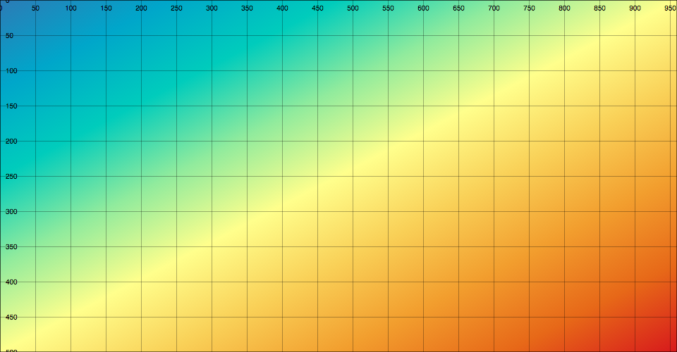 The zoom behavior can be combined with other behaviors, such as d3-drag for dragging, and d3-brush for focus + context.
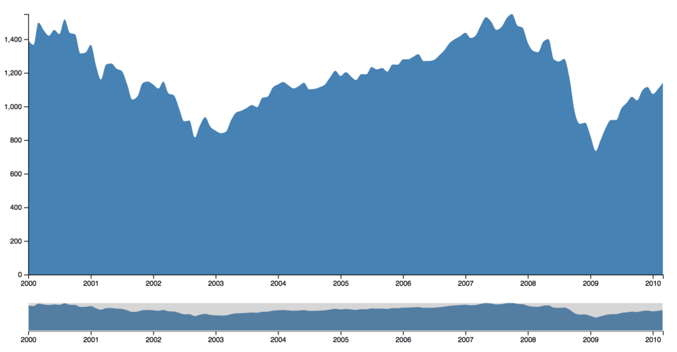 The zoom behavior can be controlled programmatically using zoom.transform, allowing you to implement user interface controls which drive the display or to stage animated tours through your data.
Smooth zoom transitions are based on “Smooth and efficient zooming and panning” by Jarke J.
van Wijk and Wim A.A.
Nuij.
The zoom behavior can be controlled programmatically using zoom.transform, allowing you to implement user interface controls which drive the display or to stage animated tours through your data.
Smooth zoom transitions are based on “Smooth and efficient zooming and panning” by Jarke J.
van Wijk and Wim A.A.
Nuij.
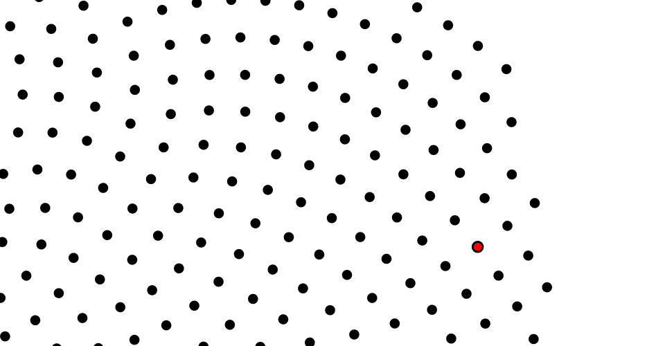 See also d3-tile for examples panning and zooming maps.
Installing
If you use NPM, npm install d3-zoom.
Otherwise, download the latest release.
You can also load directly from d3js.org, either as a standalone library or as part of D3.
AMD, CommonJS, and vanilla environments are supported.
In vanilla, a d3 global is exported:
<script src="https://d3js.org/d3-color.v2.min.js"></script>
<script src="https://d3js.org/d3-dispatch.v2.min.js"></script>
<script src="https://d3js.org/d3-ease.v2.min.js"></script>
<script src="https://d3js.org/d3-interpolate.v2.min.js"></script>
<script src="https://d3js.org/d3-selection.v2.min.js"></script>
<script src="https://d3js.org/d3-timer.v2.min.js"></script>
<script src="https://d3js.org/d3-transition.v2.min.js"></script>
<script src="https://d3js.org/d3-drag.v2.min.js"></script>
<script src="https://d3js.org/d3-zoom.v2.min.js"></script>
<script>
var zoom = d3.zoom();
</script>
Try d3-zoom in your browser.
API Reference
This table describes how the zoom behavior interprets native events:
| Event |
Listening Element |
Zoom Event |
Default Prevented? |
| mousedown5 |
selection |
start |
no¹ |
| mousemove² |
window¹ |
zoom |
yes |
| mouseup² |
window¹ |
end |
yes |
| dragstart² |
window |
- |
yes |
| selectstart² |
window |
- |
yes |
| click³ |
window |
- |
yes |
| dblclick |
selection |
multiple6 |
yes |
| wheel8 |
selection |
zoom7 |
yes |
| touchstart |
selection |
multiple6 |
no4 |
| touchmove |
selection |
zoom |
yes |
| touchend |
selection |
end |
no4 |
| touchcancel |
selection |
end |
no4 |
The propagation of all consumed events is immediately stopped.
¹ Necessary to capture events outside an iframe; see d3-drag#9.
² Only applies during an active, mouse-based gesture; see d3-drag#9.
³ Only applies immediately after some mouse-based gestures; see zoom.clickDistance.
4 Necessary to allow click emulation on touch input; see d3-drag#9.
5 Ignored if within 500ms of a touch gesture ending; assumes click emulation.
6 Double-click and double-tap initiate a transition that emits start, zoom and end events; see zoom.tapDistance..
7 The first wheel event emits a start event; an end event is emitted when no wheel events are received for 150ms.
8 Ignored if already at the corresponding limit of the scale extent.
# d3.zoom() · Source, Examples
Creates a new zoom behavior.
The returned behavior, zoom, is both an object and a function, and is typically applied to selected elements via selection.call.
# zoom(selection) · Source, Examples
Applies this zoom behavior to the specified selection, binding the necessary event listeners to allow panning and zooming, and initializing the zoom transform on each selected element to the identity transform if not already defined.
This function is typically not invoked directly, and is instead invoked via selection.call.
For example, to instantiate a zoom behavior and apply it to a selection:
selection.call(d3.zoom().on("zoom", zoomed));
Internally, the zoom behavior uses selection.on to bind the necessary event listeners for zooming.
The listeners use the name .zoom, so you can subsequently unbind the zoom behavior as follows:
selection.on(".zoom", null);
To disable just wheel-driven zooming (say to not interfere with native scrolling), you can remove the zoom behavior’s wheel event listener after applying the zoom behavior to the selection:
selection
.call(zoom)
.on("wheel.zoom", null);
Alternatively, use zoom.filter for greater control over which events can initiate zoom gestures.
Applying the zoom behavior also sets the -webkit-tap-highlight-color style to transparent, disabling the tap highlight on iOS.
If you want a different tap highlight color, remove or re-apply this style after applying the drag behavior.
# zoom.transform(selection, transform[, point]) · Source, Examples
If selection is a selection, sets the current zoom transform of the selected elements to the specified transform, instantaneously emitting start, zoom and end events.
If selection is a transition, defines a “zoom” tween to the specified transform using d3.interpolateZoom, emitting a start event when the transition starts, zoom events for each tick of the transition, and then an end event when the transition ends (or is interrupted).
The transition will attempt to minimize the visual movement around the specified point; if the point is not specified, it defaults to the center of the viewport extent.
The transform may be specified either as a zoom transform or as a function that returns a zoom transform; similarly, the point may be specified either as a two-element array [x, y] or a function that returns such an array.
If a function, it is invoked for each selected element, being passed the current event (event) and datum d, with the this context as the current DOM element.
This function is typically not invoked directly, and is instead invoked via selection.call or transition.call.
For example, to reset the zoom transform to the identity transform instantaneously:
selection.call(zoom.transform, d3.zoomIdentity);
To smoothly reset the zoom transform to the identity transform over 750 milliseconds:
selection.transition().duration(750).call(zoom.transform, d3.zoomIdentity);
This method requires that you specify the new zoom transform completely, and does not enforce the defined scale extent and translate extent, if any.
To derive a new transform from the existing transform, and to enforce the scale and translate extents, see the convenience methods zoom.translateBy, zoom.scaleBy and zoom.scaleTo.
# zoom.translateBy(selection, x, y) · Source
If selection is a selection, translates the current zoom transform of the selected elements by x and y, such that the new tx1 = tx0 + kx and ty1 = ty0 + ky.
If selection is a transition, defines a “zoom” tween translating the current transform.
This method is a convenience method for zoom.transform.
The x and y translation amounts may be specified either as numbers or as functions that return numbers.
If a function, it is invoked for each selected element, being passed the current datum d and index i, with the this context as the current DOM element.
# zoom.translateTo(selection, x, y[, p]) · Source
If selection is a selection, translates the current zoom transform of the selected elements such that the given position x,y appears at given point p.
The new tx = px - kx and ty = py - ky.
If p is not specified, it defaults to the center of the viewport extent.
If selection is a transition, defines a “zoom” tween translating the current transform.
This method is a convenience method for zoom.transform.
The x and y coordinates may be specified either as numbers or as functions that returns numbers; similarly the p point may be specified either as a two-element array [px,py] or a function.
If a function, it is invoked for each selected element, being passed the current datum d and index i, with the this context as the current DOM element.
# zoom.scaleBy(selection, k[, p]) · Source
If selection is a selection, scales the current zoom transform of the selected elements by k, such that the new k1 = k0k.
The reference point p does move.
If p is not specified, it defaults to the center of the viewport extent.
If selection is a transition, defines a “zoom” tween translating the current transform.
This method is a convenience method for zoom.transform.
The k scale factor may be specified either as a number or a function that returns a number; similarly the p point may be specified either as a two-element array [px,py] or a function.
If a function, it is invoked for each selected element, being passed the current datum d and index i, with the this context as the current DOM element.
# zoom.scaleTo(selection, k[, p]) · Source
If selection is a selection, scales the current zoom transform of the selected elements to k, such that the new k1 = k.
The reference point p does move.
If p is not specified, it defaults to the center of the viewport extent.
If selection is a transition, defines a “zoom” tween translating the current transform.
This method is a convenience method for zoom.transform.
The k scale factor may be specified either as a number or a function that returns a number; similarly the p point may be specified either as a two-element array [px,py] or a function.
If a function, it is invoked for each selected element, being passed the current datum d and index i, with the this context as the current DOM element.
# zoom.constrain([constrain]) · Source
If constrain is specified, sets the transform constraint function to the specified function and returns the zoom behavior.
If constrain is not specified, returns the current constraint function, which defaults to:
function constrain(transform, extent, translateExtent) {
var dx0 = transform.invertX(extent[0][0]) - translateExtent[0][0],
dx1 = transform.invertX(extent[1][0]) - translateExtent[1][0],
dy0 = transform.invertY(extent[0][1]) - translateExtent[0][1],
dy1 = transform.invertY(extent[1][1]) - translateExtent[1][1];
return transform.translate(
dx1 > dx0 ? (dx0 + dx1) / 2 : Math.min(0, dx0) || Math.max(0, dx1),
dy1 > dy0 ? (dy0 + dy1) / 2 : Math.min(0, dy0) || Math.max(0, dy1)
);
}
The constraint function must return a transform given the current transform, viewport extent and translate extent.
The default implementation attempts to ensure that the viewport extent does not go outside the translate extent.
# zoom.filter([filter]) · Source
If filter is specified, sets the filter to the specified function and returns the zoom behavior.
If filter is not specified, returns the current filter, which defaults to:
function filter(event) {
return !event.ctrlKey && !event.button;
}
The filter is passed the current event (event) and datum d, with the this context as the current DOM element.
If the filter returns falsey, the initiating event is ignored and no zoom gestures are started.
Thus, the filter determines which input events are ignored.
The default filter ignores mousedown events on secondary buttons, since those buttons are typically intended for other purposes, such as the context menu.
# zoom.touchable([touchable]) · Source
If touchable is specified, sets the touch support detector to the specified function and returns the zoom behavior.
If touchable is not specified, returns the current touch support detector, which defaults to:
function touchable() {
return navigator.maxTouchPoints || ("ontouchstart" in this);
}
Touch event listeners are only registered if the detector returns truthy for the corresponding element when the zoom behavior is applied.
The default detector works well for most browsers that are capable of touch input, but not all; Chrome’s mobile device emulator, for example, fails detection.
# zoom.wheelDelta([delta]) · Source
If delta is specified, sets the wheel delta function to the specified function and returns the zoom behavior.
If delta is not specified, returns the current wheel delta function, which defaults to:
function wheelDelta(event) {
return -event.deltaY * (event.deltaMode === 1 ? 0.05 : event.deltaMode ? 1 : 0.002);
}
The value returned by the wheel delta function determines the amount of scaling applied in response to a WheelEvent.
The scale factor transform.k is multiplied by 2; for example, a of +1 doubles the scale factor, of -1 halves the scale factor.
# zoom.extent([extent]) · Source
If extent is specified, sets the viewport extent to the specified array of points [[x0, y0], [x1, y1]], where [x0, y0] is the top-left corner of the viewport and [x1, y1] is the bottom-right corner of the viewport, and returns this zoom behavior.
The extent may also be specified as a function which returns such an array; if a function, it is invoked for each selected element, being passed the current datum d, with the this context as the current DOM element.
If extent is not specified, returns the current extent accessor, which defaults to [[0, 0], [width, height]] where width is the client width of the element and height is its client height; for SVG elements, the nearest ancestor SVG element’s viewBox, or width and height attributes, are used.
Alternatively, consider using element.getBoundingClientRect.
The viewport extent affects several functions: the center of the viewport remains fixed during changes by zoom.scaleBy and zoom.scaleTo; the viewport center and dimensions affect the path chosen by d3.interpolateZoom; and the viewport extent is needed to enforce the optional translate extent.
# zoom.scaleExtent([extent]) · Source
If extent is specified, sets the scale extent to the specified array of numbers [k0, k1] where k0 is the minimum allowed scale factor and k1 is the maximum allowed scale factor, and returns this zoom behavior.
If extent is not specified, returns the current scale extent, which defaults to [0, 8].
The scale extent restricts zooming in and out.
It is enforced on interaction and when using zoom.scaleBy, zoom.scaleTo and zoom.translateBy; however, it is not enforced when using zoom.transform to set the transform explicitly.
If the user tries to zoom by wheeling when already at the corresponding limit of the scale extent, the wheel events will be ignored and not initiate a zoom gesture.
This allows the user to scroll down past a zoomable area after zooming in, or to scroll up after zooming out.
If you would prefer to always prevent scrolling on wheel input regardless of the scale extent, register a wheel event listener to prevent the browser default behavior:
selection
.call(zoom)
.on("wheel", event => event.preventDefault());
# zoom.translateExtent([extent]) · Source
If extent is specified, sets the translate extent to the specified array of points [[x0, y0], [x1, y1]], where [x0, y0] is the top-left corner of the world and [x1, y1] is the bottom-right corner of the world, and returns this zoom behavior.
If extent is not specified, returns the current translate extent, which defaults to [[-8, -8], [+8, +8]].
The translate extent restricts panning, and may cause translation on zoom out.
It is enforced on interaction and when using zoom.scaleBy, zoom.scaleTo and zoom.translateBy; however, it is not enforced when using zoom.transform to set the transform explicitly.
# zoom.clickDistance([distance]) · Source
If distance is specified, sets the maximum distance that the mouse can move between mousedown and mouseup that will trigger a subsequent click event.
If at any point between mousedown and mouseup the mouse is greater than or equal to distance from its position on mousedown, the click event following mouseup will be suppressed.
If distance is not specified, returns the current distance threshold, which defaults to zero.
The distance threshold is measured in client coordinates (event.clientX and event.clientY).
# zoom.tapDistance([distance]) · Source
If distance is specified, sets the maximum distance that a double-tap gesture can move between first touchstart and second touchend that will trigger a subsequent double-click event.
If distance is not specified, returns the current distance threshold, which defaults to 10.
The distance threshold is measured in client coordinates (event.clientX and event.clientY).
# zoom.duration([duration]) · Source
If duration is specified, sets the duration for zoom transitions on double-click and double-tap to the specified number of milliseconds and returns the zoom behavior.
If duration is not specified, returns the current duration, which defaults to 250 milliseconds.
If the duration is not greater than zero, double-click and -tap trigger instantaneous changes to the zoom transform rather than initiating smooth transitions.
To disable double-click and double-tap transitions, you can remove the zoom behavior’s dblclick event listener after applying the zoom behavior to the selection:
selection
.call(zoom)
.on("dblclick.zoom", null);
# zoom.interpolate([interpolate]) · Source
If interpolate is specified, sets the interpolation factory for zoom transitions to the specified function.
If interpolate is not specified, returns the current interpolation factory, which defaults to d3.interpolateZoom to implement smooth zooming.
To apply direct interpolation between two views, try d3.interpolate instead.
# zoom.on(typenames[, listener]) · Source
If listener is specified, sets the event listener for the specified typenames and returns the zoom behavior.
If an event listener was already registered for the same type and name, the existing listener is removed before the new listener is added.
If listener is null, removes the current event listeners for the specified typenames, if any.
If listener is not specified, returns the first currently-assigned listener matching the specified typenames, if any.
When a specified event is dispatched, each listener will be invoked with the same context and arguments as selection.on listeners: the current event (event) and datum d, with the this context as the current DOM element.
The typenames is a string containing one or more typename separated by whitespace.
Each typename is a type, optionally followed by a period (.) and a name, such as zoom.foo and zoom.bar; the name allows multiple listeners to be registered for the same type.
The type must be one of the following:
start - after zooming begins (such as on mousedown).
zoom - after a change to the zoom transform (such as on mousemove).
end - after zooming ends (such as on mouseup ).
See dispatch.on for more.
Zoom Events
When a zoom event listener is invoked, it receives the current zoom event as a first argument.
The event object exposes several fields:
event.target - the associated zoom behavior.
event.type - the string “start”, “zoom” or “end”; see zoom.on.
event.transform - the current zoom transform.
event.sourceEvent - the underlying input event, such as mousemove or touchmove.
Zoom Transforms
The zoom behavior stores the zoom state on the element to which the zoom behavior was applied, not on the zoom behavior itself.
This is because the zoom behavior can be applied to many elements simultaneously, and each element can be zoomed independently.
The zoom state can change either on user interaction or programmatically via zoom.transform.
To retrieve the zoom state, use event.transform on the current zoom event within a zoom event listener (see zoom.on), or use d3.zoomTransform for a given node.
The latter is particularly useful for modifying the zoom state programmatically, say to implement buttons for zooming in and out.
# d3.zoomTransform(node) · Source
Returns the current transform for the specified node.
Note that node should typically be a DOM element, not a selection.
(A selection may consist of multiple nodes, in different states, and this function only returns a single transform.) If you have a selection, call selection.node first:
var transform = d3.zoomTransform(selection.node());
In the context of an event listener, the node is typically the element that received the input event (which should be equal to event.transform), this:
var transform = d3.zoomTransform(this);
Internally, an element’s transform is stored as element.__zoom; however, you should use this method rather than accessing it directly.
If the given node has no defined transform, returns the transform of the closest ancestor, or if none exists, the identity transformation.
The returned transform represents a two-dimensional transformation matrix of the form:
k 0 tx
0 k ty
0 0 1
(This matrix is capable of representing only scale and translation; a future release may also allow rotation, though this would probably not be a backwards-compatible change.) The position x,y is transformed to xk + tx,yk + ty.
The transform object exposes the following properties:
transform.x - the translation amount tx along the x-axis.
transform.y - the translation amount ty along the y-axis.
transform.k - the scale factor k.
These properties should be considered read-only; instead of mutating a transform, use transform.scale and transform.translate to derive a new transform.
Also see zoom.scaleBy, zoom.scaleTo and zoom.translateBy for convenience methods on the zoom behavior.
To create a transform with a given k, tx, and ty:
var t = d3.zoomIdentity.translate(x, y).scale(k);
To apply the transformation to a Canvas 2D context, use context.translate followed by context.scale:
context.translate(transform.x, transform.y);
context.scale(transform.k, transform.k);
Similarly, to apply the transformation to HTML elements via CSS:
div.style("transform", "translate(" + transform.x + "px," + transform.y + "px) scale(" + transform.k + ")");
div.style("transform-origin", "0 0");
To apply the transformation to SVG:
g.attr("transform", "translate(" + transform.x + "," + transform.y + ") scale(" + transform.k + ")");
Or more simply, taking advantage of transform.toString:
g.attr("transform", transform);
Note that the order of transformations matters! The translate must be applied before the scale.
# transform.scale(k) · Source
Returns a transform whose scale k1 is equal to k0k, where k0 is this transform’s scale.
# transform.translate(x, y) · Source
Returns a transform whose translation tx1 and ty1 is equal to tx0 + tk x and ty0 + tk y, where tx0 and ty0 is this transform’s translation and tk is this transform’s scale.
# transform.apply(point) · Source
Returns the transformation of the specified point which is a two-element array of numbers [x, y].
The returned point is equal to [xk + tx, yk + ty].
# transform.applyX(x) · Source
Returns the transformation of the specified x-coordinate, xk + tx.
# transform.applyY(y) · Source
Returns the transformation of the specified y-coordinate, yk + ty.
# transform.invert(point) · Source
Returns the inverse transformation of the specified point which is a two-element array of numbers [x, y].
The returned point is equal to [(x - tx) / k, (y - ty) / k].
# transform.invertX(x) · Source
Returns the inverse transformation of the specified x-coordinate, (x - tx) / k.
# transform.invertY(y) · Source
Returns the inverse transformation of the specified y-coordinate, (y - ty) / k.
# transform.rescaleX(x) · Source
Returns a copy of the continuous scale x whose domain is transformed.
This is implemented by first applying the inverse x-transform on the scale’s range, and then applying the inverse scale to compute the corresponding domain:
function rescaleX(x) {
var range = x.range().map(transform.invertX, transform),
domain = range.map(x.invert, x);
return x.copy().domain(domain);
}
The scale x must use d3.interpolateNumber; do not use continuous.rangeRound as this reduces the accuracy of continuous.invert and can lead to an inaccurate rescaled domain.
This method does not modify the input scale x; x thus represents the untransformed scale, while the returned scale represents its transformed view.
# transform.rescaleY(y) · Source
Returns a copy of the continuous scale y whose domain is transformed.
This is implemented by first applying the inverse y-transform on the scale’s range, and then applying the inverse scale to compute the corresponding domain:
function rescaleY(y) {
var range = y.range().map(transform.invertY, transform),
domain = range.map(y.invert, y);
return y.copy().domain(domain);
}
The scale y must use d3.interpolateNumber; do not use continuous.rangeRound as this reduces the accuracy of continuous.invert and can lead to an inaccurate rescaled domain.
This method does not modify the input scale y; y thus represents the untransformed scale, while the returned scale represents its transformed view.
# transform.toString() · Source
Returns a string representing the SVG transform corresponding to this transform.
Implemented as:
function toString() {
return "translate(" + this.x + "," + this.y + ") scale(" + this.k + ")";
}
# d3.zoomIdentity · Source
The identity transform, where k = 1, tx = ty = 0.

